Z-Curve Publication Bias Diagnostics
František Bartoš
2025-12-18
Source:vignettes/ZCurveDiagnostics.Rmd
ZCurveDiagnostics.RmdIntroduction
This vignette accompanies the “Z-Curve Plot: A Visual Diagnostic for Publication Bias in Meta-Analysis” manuscript (Bartoš & Schimmack, 2025). The manuscript provides the theoretical foundation and detailed methodology for z-curve diagnostics, while this vignette demonstrates their practical implementation using the RoBMA R package (Bartoš & Maier, 2020).
Z-curve plots provide a visual assessment of meta-analytic model fit specifically aimed at detecting misfit due to publication bias (Bartoš & Schimmack, 2025). The methodology overlays model-implied posterior predictive distributions of z-statistics on the observed distribution of z-statistics (Gabry et al., 2019), allowing researchers to assess how well different meta-analytic models capture the patterns in their data. The approach builds on the z-curve methodology developed by Brunner & Schimmack (2020) for assessing the quality of research.
The z-curve approach complements statistical tests of publication bias (such as inclusion Bayes factors) with intuitive visualizations that can highlight model misfit due to publication bias. Additionally, the method allows extrapolation to the pre-publication bias state, providing estimates of key metrics such as the expected discovery rate and the number of missing studies.
We illustrate the z-curve diagnostics using four empirical examples from recent meta-analyses that exhibit different degrees of publication bias. The examples demonstrate how to interpret z-curve plots and use them to guide model selection in meta-analytic practice. For details refer to the accompanying manuscript (Bartoš & Schimmack, 2025).
Getting Started
Before we start, we load the RoBMA package:
The z-curve diagnostic workflow consists of the following steps:
- Fit meta-analytic models to your data using
NoBMA()for random-effects models orRoBMA()for publication bias-adjusted models (Bartoš et al., 2023; Maier et al., 2023). - Create z-curve objects using the
as_zcurve()function. - Generate histograms of observed z-statistics using
hist(). - Overlay model fits using
lines()to compare different models. - Use the visualization to supplement statistical model comparison.
Note that when using NoBMA() to fit a standard
random-effects model we need to set
priors_effect_null = NULL and
priors_heterogeneity_null = NULL to disable model averaging
across null hypotheses. This ensures we fit a single random-effects
model rather than a Bayesian model-averaged ensemble. The z-curve plot
is implemented only for models fitted using the spike-and-slab algorithm
specified via algorithm = "ss".
Applied Examples
We demonstrate the z-curve diagnostics on four empirical meta-analyses that represent different publication bias scenarios:
- Ease-of-retrieval effect in the few/many paradigm (Weingarten & Hutchinson, 2018) - An example with extreme publication bias
- Social comparison as behavior change technique (Hoppen et al., 2025) - An example with strong publication bias
-
ChatGPT effects on learning performance (Wang & Fan, 2025) - An example with
moderate publication bias
- Framing effects from Many Labs 2 (Klein et al., 2018) - An example with no publication bias (registered replication reports)
For each example, we fit both a simple random-effects model using
NoBMA() and a publication bias-adjusted ensemble using
RoBMA() (Bartoš et al., 2023; Maier
et al., 2023). We then use z-curve plots to compare how well each
model captures the observed distribution of z-statistics.
Example 1: Ease-of-Retrieval Effect in the Few/Many Paradigm
This example examines the ease-of-retrieval effect, a well-established phenomenon in cognitive psychology where the subjective difficulty of recalling information influences judgments more than the actual number of items recalled (schwarz1991ease?).
We analyze 298 estimates from 111 studies examining the ease-of-retrieval effect in the few/many standard paradigm in the proximal dataset collected by Weingarten and colleagues (Weingarten & Hutchinson, 2018). The original analysis reported a pooled effect size r = 0.25, 95% CI [0.22, 0.28]. When adjusted for publication bias using PET-PEESE, the effect was reduced but remained substantial at r = 0.19, 95% CI [0.15, 0.23].
Data and Model Fitting
We begin by loading the ease-of-retrieval dataset and examining its structure. We focus on studies using the standard paradigm in proximal dataset conditions:
# Load the ease-of-retrieval dataset
data("Weingarten2018", package = "RoBMA")
# Filter to standard paradigm and proximal dataset as in the original analysis
Weingarten2018 <- Weingarten2018[Weingarten2018$standard_paradigm & Weingarten2018$proximal_dataset, ]
head(Weingarten2018)
#>          r_xy    N paper_id published   USA number_of_few number_of_many
#> 129 0.2921094 20.0        1      TRUE FALSE             6             12
#> 130 0.2675424 20.0        1      TRUE FALSE             6             12
#> 131 0.1741571 79.0        1      TRUE FALSE             6             12
#> 132 0.2076078 79.0        1      TRUE FALSE             6             12
#> 135 0.3333333 19.5        1      TRUE FALSE             6             12
#> 136 0.3855344 19.5        1      TRUE FALSE             6             12
#>     episodic_memory standard_paradigm proximal_dataset      r_xm  r_my
#> 129            TRUE              TRUE             TRUE 0.3232300  0.35
#> 130            TRUE              TRUE             TRUE 0.3232300  0.66
#> 131            TRUE              TRUE             TRUE 0.1879524  0.12
#> 132            TRUE              TRUE             TRUE 0.1879524  0.32
#> 135            TRUE              TRUE             TRUE 0.1566084 -0.03
#> 136            TRUE              TRUE             TRUE 0.1566084  0.23
The filtered dataset contains 298 effect size estimates (correlation
coefficients) and sample sizes. Since the effect size estimates are
nested within studies (indicated by the paper_id variable),
we specify a multilevel random-effects model using NoBMA()
and a multilevel publication bias-adjusted model using
RoBMA() (Bartoš et al.,
2025). (Note that RoBMA internally transforms the correlation
coefficients to Fisher’s z for analysis.)
# Fit random-effects model (unadjusted for publication bias)
fit_RE_Weingarten2018 <- NoBMA(r = Weingarten2018$r_xy, n = round(Weingarten2018$N),
                               study_ids = Weingarten2018$paper_id,
                               priors_effect_null = NULL, priors_heterogeneity_null = NULL,
                               algorithm = "ss", sample = 10000, burnin = 10000, adapt = 10000,
                               chains = 5, parallel = TRUE, seed = 1)

# Fit RoBMA model (adjusted for publication bias)
fit_RoBMA_Weingarten2018 <- RoBMA(r = Weingarten2018$r_xy, n = round(Weingarten2018$N),
                                  study_ids = Weingarten2018$paper_id,
                                  algorithm = "ss", sample = 10000, burnin = 10000, adapt = 10000,
                                  chains = 5, parallel = TRUE, seed = 1)
Model Results Summary
We can examine the results from both models using the
summary() function.
# Random-effects model results
summary(fit_RE_Weingarten2018, output_scale = "r")
#> Call:
#> RoBMA(d = d, r = r, logOR = logOR, OR = OR, z = z, y = y, se = se,
#>     v = v, n = n, lCI = lCI, uCI = uCI, t = t, study_names = study_names,
#>     study_ids = study_ids, data = data, transformation = transformation,
#>     prior_scale = prior_scale, effect_direction = "positive",
#>     model_type = model_type, priors_effect = priors_effect, priors_heterogeneity = priors_heterogeneity,
#>     priors_bias = NULL, priors_effect_null = priors_effect_null,
#>     priors_heterogeneity_null = priors_heterogeneity_null, priors_bias_null = prior_none(),
#>     priors_hierarchical = priors_hierarchical, priors_hierarchical_null = priors_hierarchical_null,
#>     algorithm = algorithm, chains = chains, sample = sample,
#>     burnin = burnin, adapt = adapt, thin = thin, parallel = parallel,
#>     autofit = autofit, autofit_control = autofit_control, convergence_checks = convergence_checks,
#>     save = save, seed = seed, silent = silent)
#>
#> Bayesian model-averaged meta-analysis (normal-normal model)
#> Components summary:
#>               Prior prob. Post. prob. Inclusion BF
#> Effect              1.000       1.000          Inf
#> Heterogeneity       1.000       1.000          Inf
#> Hierarchical        1.000       1.000          Inf
#>
#> Model-averaged estimates:
#>      Mean Median 0.025 0.975
#> mu  0.246  0.246 0.220 0.273
#> tau 0.120  0.120 0.097 0.148
#> rho 0.946  0.955 0.844 0.997
#> The effect size estimates are summarized on the correlation scale and heterogeneity is summarized on the Fisher's z scale (priors were specified on the Cohen's d scale).
#> (Estimated publication weights omega correspond to one-sided p-values.)

# RoBMA model results
summary(fit_RoBMA_Weingarten2018, output_scale = "r")
#> Call:
#> RoBMA(r = Weingarten2018$r_xy, n = round(Weingarten2018$N), study_ids = Weingarten2018$paper_id,
#>     algorithm = "ss", chains = 5, sample = 10000, burnin = 10000,
#>     adapt = 10000, parallel = TRUE, save = "min", seed = 1)
#>
#> Robust Bayesian meta-analysis
#> Components summary:
#>               Prior prob. Post. prob. Inclusion BF
#> Effect              0.500       1.000          Inf
#> Heterogeneity       0.500       1.000          Inf
#> Bias                0.500       1.000          Inf
#> Hierarchical        1.000       1.000          Inf
#>
#> Model-averaged estimates:
#>                    Mean Median 0.025 0.975
#> mu                0.170  0.170 0.131 0.208
#> tau               0.128  0.128 0.100 0.160
#> rho               0.959  0.967 0.877 0.998
#> omega[0,0.025]    1.000  1.000 1.000 1.000
#> omega[0.025,0.05] 0.882  0.927 0.587 1.000
#> omega[0.05,0.5]   0.273  0.268 0.169 0.409
#> omega[0.5,0.95]   0.099  0.091 0.038 0.207
#> omega[0.95,0.975] 0.099  0.091 0.038 0.207
#> omega[0.975,1]    0.099  0.091 0.038 0.207
#> PET               0.000  0.000 0.000 0.000
#> PEESE             0.000  0.000 0.000 0.000
#> The effect size estimates are summarized on the correlation scale and heterogeneity is summarized on the Fisher's z scale (priors were specified on the Cohen's d scale).
#> (Estimated publication weights omega correspond to one-sided p-values.)
The Bayesian multilevel random-effects model finds results similar to those reported in the original publication-bias-unadjusted analysis.
The RoBMA analysis reveals extreme evidence for publication bias. However, RoBMA still finds extreme evidence for the presence of an effect, with a model-averaged effect size estimate of g = 0.17, 95% CI [0.13, 0.21].
Creating Z-Curve Objects
The as_zcurve() function converts fitted RoBMA models
into objects suitable for z-curve visualization:
Z-Curve Diagnostic Plots
We now generate z-curve plots to assess how well each model captures
the observed distribution of z-statistics. The hist()
function creates a histogram of the observed z-statistics, while
lines() overlays the model-implied posterior predictive
distributions (Gabry et al., 2019):
# Create histogram of observed z-statistics
hist(zcurve_RoBMA_Weingarten2018, from = -3, to = 6, by = 0.25)

# Add model-implied distributions
lines(zcurve_RE_Weingarten2018, from = -3, to = 6, col = "black", lty = 2, lwd = 2)
lines(zcurve_RoBMA_Weingarten2018, from = -3, to = 6, col = "blue", lty = 2, lwd = 2)

# Add legend
legend("topright",
       legend = c("Random-Effects", "RoBMA"),
       col = c("black", "blue"),
       lty = 2, lwd = 2)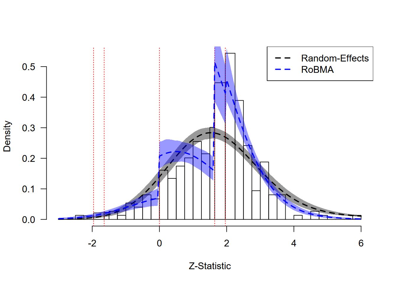
Ease-of-Retrieval Effect: Model Fit Assessment
The z-curve plot reveals clear evidence of extreme publication bias in the ease-of-retrieval literature. Two extreme discontinuities are visible in the observed distribution of z-statistics (gray bars):
Marginal Significance Threshold (z ≈ 1.64): There is a sharp increase in the frequency of test statistics just above the threshold for marginal significance (α = 0.10).
Zero Threshold (z = 0): A weaker discontinuity occurs at zero, with additional suppression of studies reporting negative effects (z < 0).
The random-effects model (black dashed line) fails to capture these patterns. It systematically overestimates the number of negative results and non-significant positive results.
RoBMA (blue dashed line) captures both discontinuities and approximates the observed data much better. These results provide extreme evidence for the presence of publication bias and highlight the need to interpret the publication bias-adjusted model.
Extrapolation to Pre-Publication Bias
The package also allows us to extrapolate what the distribution of
z-statistics might have looked like in the absence of publication bias.
This is achieved by calling the plot() function (with the
default plot_extrapolation = TRUE argument).
# Plot extrapolation to pre-publication bias
plot(zcurve_RoBMA_Weingarten2018, from = -3, to = 6, by.hist = 0.25)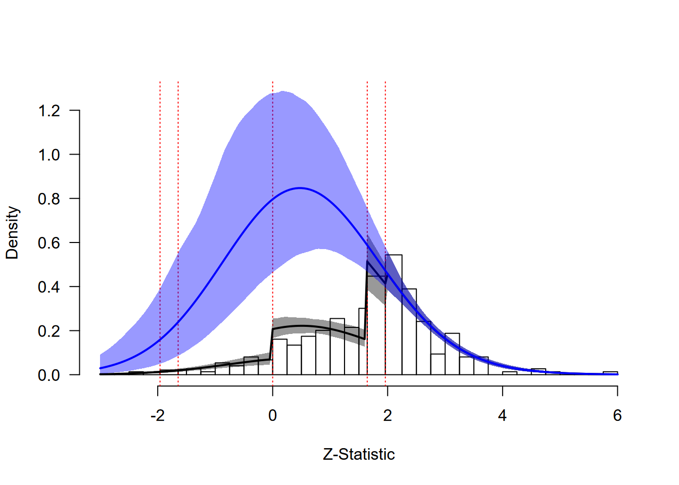
Ease-of-Retrieval Effect: Extrapolation Analysis
The extrapolated distribution (blue line) shows what we would expect to observe if studies were published regardless of their results. Comparing the fitted distribution (accounting for publication bias) with the extrapolated distribution reveals the extent of the bias. The large discrepancy between these distributions quantifies the substantial impact of publication bias in this literature.
Z-Curve Summary Metrics
This discrepancy can be summarized with the additional statistics
provided by the summary() function.
# Extract z-curve summary metrics
summary(zcurve_RoBMA_Weingarten2018)
#> Call:
#> as_zcurve: RoBMA(r = Weingarten2018$r_xy, n = round(Weingarten2018$N), study_ids = Weingarten2018$paper_id,
#>     algorithm = "ss", chains = 5, sample = 10000, burnin = 10000,
#>     adapt = 10000, parallel = TRUE, save = "min", seed = 1)
#>
#> Z-curve
#> Model-averaged estimates:
#>              Mean  Median   0.025    0.975
#> EDR         0.187   0.184   0.144    0.236
#> Soric FDR   0.234   0.233   0.170    0.312
#> Missing N 561.951 525.437 277.430 1068.835
#> Estimated using 298 estimates, 134 significant (ODR = 0.45, 95 CI [0.39, 0.51]).
The summary provides several key results: The observed discovery rate (ODR = 0.45) substantially exceeds the expected discovery rate (EDR = 0.18, 95% CI [0.14, 0.23]), indicating that roughly 2.5 times as many significant results appear in the published literature as we would expect. The estimated number of missing studies, 579 (95% CI [311, 1014]), suggests that a substantial number of non-significant or negative results may be absent from the published literature. The false discovery risk (FDR = 0.24, 95% CI [0.18, 0.31]) provides an upper bound on the proportion of statistically significant results that may be false positives, though this risk remains moderate due to evidence for a genuine underlying effect despite the extreme publication bias.
Example 2: Social Comparison and Behavior Change
This example examines a meta-analysis of randomized controlled trials evaluating the efficacy of social comparison as a behavior change technique (Hoppen et al., 2025). The analysis includes 37 trials comparing social comparison interventions to passive controls across domains including climate-change mitigation, health, performance, and service outcomes.
Data and Model Fitting
Again, we begin by loading the social comparison dataset and examining its structure:
# Load the social comparison dataset
data("Hoppen2025", package = "RoBMA")
head(Hoppen2025)
#>           d            v        outcome feedback_level  social_comparison_type
#> 1 0.2206399 3.043547e-02    performance     individual             performance
#> 2 0.1284494 5.946958e-03 sustainability          group          sustainability
#> 3 0.1187558 7.707186e-04 sustainability          group          sustainability
#> 4 0.4400000 6.968339e-05    performance          group                  safety
#> 5 0.4198868 4.756183e-02 sustainability          group monetary/sustainability
#> 6 0.0861236 2.219765e-02 sustainability          group          sustainability
#>   sessions      sample_type sample_size country
#> 1        2            other         179  Canada
#> 2        1 population-based        1035     USA
#> 3        2 population-based       21151     USA
#> 4        1 population-based      395204   China
#> 5        4          student         553  Taiwan
#> 6       NA population-based         390     USA
The dataset contains effect sizes (d) and sampling
variances (v) from individual studies. We fit both a
random-effects model using NoBMA() and a publication
bias-adjusted model using RoBMA():
# Fit random-effects model (unadjusted for publication bias)
fit_RE_Hoppen2025 <- NoBMA(d = Hoppen2025$d, se = sqrt(Hoppen2025$v),
                           priors_effect_null = NULL, priors_heterogeneity_null = NULL,
                           algorithm = "ss", sample = 10000, burnin = 5000, adapt = 5000,
                           chains = 5, parallel = TRUE, seed = 1)

# Fit RoBMA model (adjusted for publication bias)
fit_RoBMA_Hoppen2025 <- RoBMA(d = Hoppen2025$d, se = sqrt(Hoppen2025$v),
                              algorithm = "ss", sample = 10000, burnin = 5000, adapt = 5000,
                              chains = 5, parallel = TRUE, seed = 1)
Model Results Summary
We examine the key results from both models:
# Random-effects model results
summary(fit_RE_Hoppen2025)
#> Call:
#> RoBMA(d = d, r = r, logOR = logOR, OR = OR, z = z, y = y, se = se,
#>     v = v, n = n, lCI = lCI, uCI = uCI, t = t, study_names = study_names,
#>     study_ids = study_ids, data = data, transformation = transformation,
#>     prior_scale = prior_scale, effect_direction = "positive",
#>     model_type = model_type, priors_effect = priors_effect, priors_heterogeneity = priors_heterogeneity,
#>     priors_bias = NULL, priors_effect_null = priors_effect_null,
#>     priors_heterogeneity_null = priors_heterogeneity_null, priors_bias_null = prior_none(),
#>     priors_hierarchical = priors_hierarchical, priors_hierarchical_null = priors_hierarchical_null,
#>     algorithm = algorithm, chains = chains, sample = sample,
#>     burnin = burnin, adapt = adapt, thin = thin, parallel = parallel,
#>     autofit = autofit, autofit_control = autofit_control, convergence_checks = convergence_checks,
#>     save = save, seed = seed, silent = silent)
#>
#> Bayesian model-averaged meta-analysis (normal-normal model)
#> Components summary:
#>               Prior prob. Post. prob. Inclusion BF
#> Effect              1.000       1.000          Inf
#> Heterogeneity       1.000       1.000          Inf
#>
#> Model-averaged estimates:
#>      Mean Median 0.025 0.975
#> mu  0.169  0.168 0.106 0.234
#> tau 0.145  0.142 0.097 0.211
#> The estimates are summarized on the Cohen's d scale (priors were specified on the Cohen's d scale).
#> (Estimated publication weights omega correspond to one-sided p-values.)
The random-effects model estimates a positive effect size of g = 0.17, 95% CI [0.11, 0.23], suggesting a positive effect of social comparison interventions. However, this analysis does not account for potential publication bias.
# RoBMA model results
summary(fit_RoBMA_Hoppen2025)
#> Call:
#> RoBMA(d = Hoppen2025$d, se = sqrt(Hoppen2025$v), algorithm = "ss",
#>     chains = 5, sample = 10000, burnin = 5000, adapt = 5000,
#>     parallel = TRUE, save = "min", seed = 1)
#>
#> Robust Bayesian meta-analysis
#> Components summary:
#>               Prior prob. Post. prob. Inclusion BF
#> Effect              0.500       0.112        0.126
#> Heterogeneity       0.500       1.000          Inf
#> Bias                0.500       0.998      596.826
#>
#> Model-averaged estimates:
#>                     Mean Median  0.025 0.975
#> mu                -0.007  0.000 -0.152 0.046
#> tau                0.199  0.194  0.134 0.294
#> omega[0,0.025]     1.000  1.000  1.000 1.000
#> omega[0.025,0.05]  0.944  1.000  0.634 1.000
#> omega[0.05,0.5]    0.676  0.681  0.325 0.983
#> omega[0.5,0.95]    0.078  0.061  0.011 0.208
#> omega[0.95,0.975]  0.078  0.061  0.011 0.208
#> omega[0.975,1]     0.078  0.061  0.011 0.208
#> PET                0.003  0.000  0.000 0.000
#> PEESE              0.005  0.000  0.000 0.000
#> The estimates are summarized on the Cohen's d scale (priors were specified on the Cohen's d scale).
#> (Estimated publication weights omega correspond to one-sided p-values.)
When accounting for the possibility of publication bias with RoBMA, we find extreme evidence for the presence of publication bias (BF_bias = 597). Consequently, the effect size shrinks to g = -0.01, 95% CI [-0.15, 0.05], with moderate evidence against the presence of an effect (BF_effect = 0.13).
Z-Curve Diagnostic Plots
# Create z-curve objects
zcurve_RE_Hoppen2025    <- as_zcurve(fit_RE_Hoppen2025)
zcurve_RoBMA_Hoppen2025 <- as_zcurve(fit_RoBMA_Hoppen2025)
# Create histogram of observed z-statistics
hist(zcurve_RoBMA_Hoppen2025)
#> 2 z-statistics are out of the plotting range

# Add model-implied distributions
lines(zcurve_RE_Hoppen2025, col = "black", lty = 2, lwd = 2)
lines(zcurve_RoBMA_Hoppen2025, col = "blue", lty = 2, lwd = 2)

# Add legend
legend("topright",
       legend = c("Random-Effects", "RoBMA"),
       col = c("black", "blue"),
       lty = 2, lwd = 2)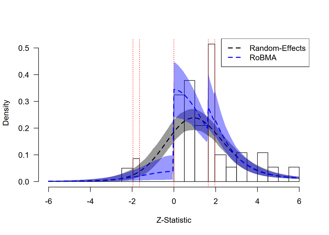
Social Comparison: Model Fit Assessment
Results
The z-curve plot highlights the clear evidence of publication bias in this dataset. We can observe pronounced discontinuities in the observed distribution (gray bars) at critical thresholds; particularly at the transition to marginal significance (z ≈ 1.64) and at zero (indicating selection against negative results).
The random-effects model (black dashed line) fails to capture these patterns, systematically overestimating the number of negative and non-significant results. In contrast, RoBMA (blue dashed line) successfully models both discontinuities, providing a markedly better fit to the observed data. This visual assessment aligns with the statistical evidence: RoBMA yields extreme evidence for publication bias and suggests that the unadjusted pooled effect is misleading.
Extrapolation to Pre-Publication Bias
The package also allows us to extrapolate what the distribution of
z-statistics might have looked like in the absence of publication bias.
This is achieved by either setting extrapolate = TRUE in
the lines() functions, or calling the plot()
function (with the default plot_extrapolation = TRUE
argument).
# Plot extrapolation to pre-publication bias
plot(zcurve_RoBMA_Hoppen2025)
#> 2 z-statistics are out of the plotting range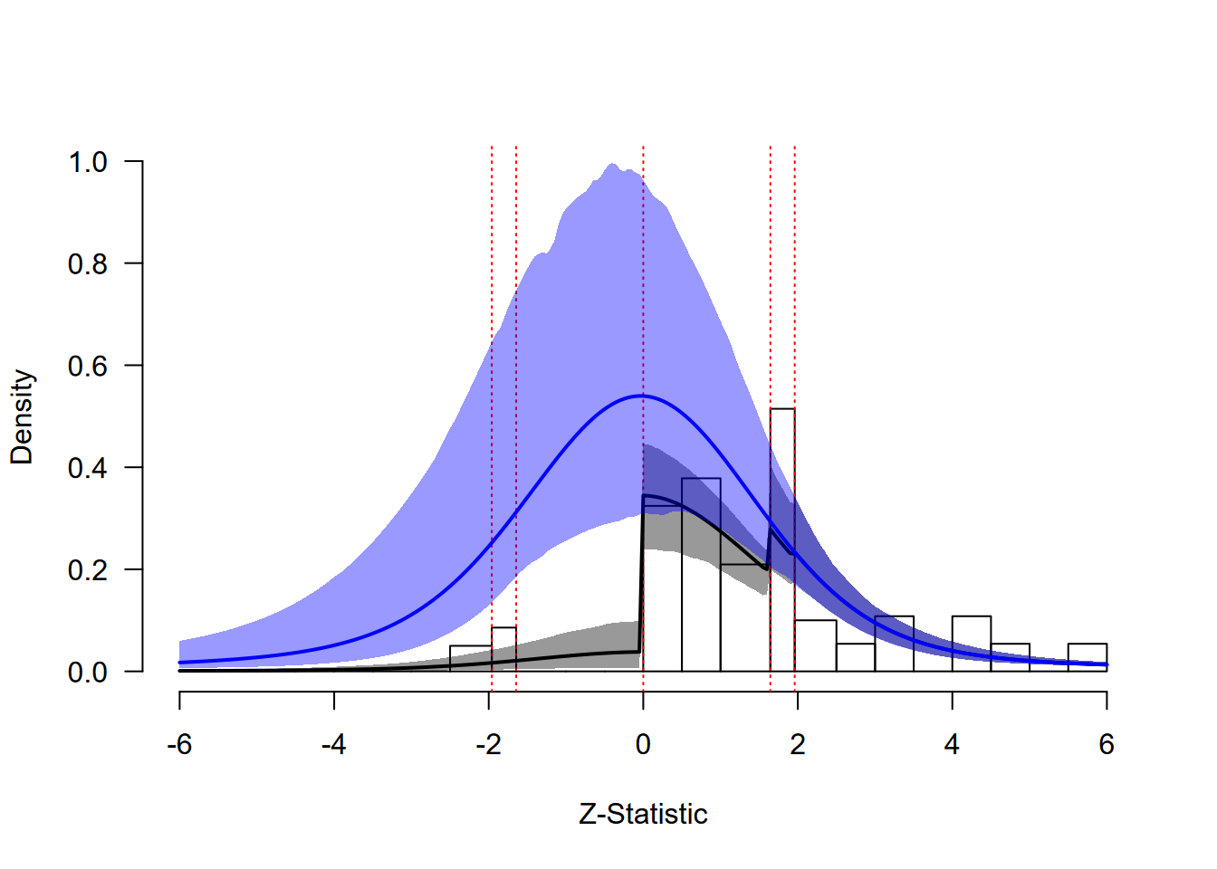
Social Comparison: Extrapolation Analysis
The extrapolated distribution (blue line) shows what we would expect to observe if studies were published regardless of their results. Comparing the fitted distribution (accounting for publication bias) with the extrapolated distribution reveals the extent of the bias. The large discrepancy between these distributions quantifies the substantial impact of publication bias in this literature, with implications for the estimated effect size and number of missing studies.
Z-Curve Summary Metrics
This discrepancy can be summarized with the additional statistics
provided by the summary() function.
# Extract z-curve summary metrics
summary(zcurve_RoBMA_Hoppen2025)
#> Call:
#> as_zcurve: RoBMA(d = Hoppen2025$d, se = sqrt(Hoppen2025$v), algorithm = "ss",
#>     chains = 5, sample = 10000, burnin = 5000, adapt = 5000,
#>     parallel = TRUE, save = "min", seed = 1)
#>
#> Z-curve
#> Model-averaged estimates:
#>             Mean Median  0.025   0.975
#> EDR        0.323  0.315  0.228   0.452
#> Soric FDR  0.116  0.114  0.064   0.178
#> Missing N 54.641 47.793 25.075 121.530
#> Estimated using 37 estimates, 12 significant (ODR = 0.32, 95 CI [0.19, 0.50]).
The summary provides several results: The observed discovery rate (ODR, i.e., the observed proportion of statistically significant results) in the dataset matches the expected discovery rate (EDR) due to the one-sided selection for marginally significant results (instead of statistically significant results). The estimated number of missing studies, 54, suggests that a considerable number of non-significant or negative results may be absent from the published literature. The false discovery risk (FDR), which corresponds to the upper bound on the false positive rate, is not extremely inflated due to the possible small positive and negative effects under the moderate heterogeneity.
Example 3: ChatGPT and Learning Performance
Our second example examines the effectiveness of ChatGPT-based interventions on students’ learning performance (Wang & Fan, 2025). This meta-analysis includes 42 randomized controlled trials comparing experimental groups (using ChatGPT for tutoring or learning support) with control groups (without ChatGPT) on learning outcomes such as exam scores and final grades.
Data Preparation and Model Fitting
We follow the same procedure as in the previous example:
# Load the ChatGPT dataset
data("Wang2025", package = "RoBMA")
# Select learning performance studies
Wang2025 <- Wang2025[Wang2025$Learning_effect == "Learning performance", ]
head(Wang2025)
#>        Learning_effect                  Author_year N_EG N_CG     g Grade_level
#> 1 Learning performance          Emran et al. (2024)   34   34 2.730     College
#> 2 Learning performance              Almohesh (2024)   75   75 1.117     Primary
#> 3 Learning performance Avello-Martnez et al. (2023)   20   21 0.062     College
#> 4 Learning performance      Boudouaia et al. (2024)   37   39 0.797     College
#> 5 Learning performance          Bai? et al. (2023a)   12   12 0.993     College
#> 6 Learning performance        Chen and Chang (2024)   31   30 1.235     College
#>                           Type_of_course Duration         Learning_model
#> 1 Language learning and academic writing  >8 week Problem-based learning
#> 2    Skills and competencies development <=1 week  Personalized learning
#> 3    Skills and competencies development <=1 week  Personalized learning
#> 4 Language learning and academic writing  >8 week    Reflective learning
#> 5               STEM and related courses <=1 week Problem-based learning
#> 6               STEM and related courses 1-4 week                  Mixed
#>             Role_of_ChatGPT Area_of_ChatGPT_application        se
#> 1 Intelligent learning tool                    Tutoring 0.3370820
#> 2         Intelligent tutor                       Mixed 0.1755723
#> 3 Intelligent learning tool Personalized recommendation 0.3125155
#> 4         Intelligent tutor   Assessment and evaluation 0.2384262
#> 5 Intelligent learning tool                    Tutoring 0.4326770
#> 6 Intelligent learning tool                       Mixed 0.2794517
# Fit models
fit_RE_Wang2025 <- NoBMA(d = Wang2025$g, se = Wang2025$se,
                         priors_effect_null = NULL, priors_heterogeneity_null = NULL,
                         algorithm = "ss", sample = 10000, burnin = 5000, adapt = 5000,
                         chains = 5, parallel = TRUE, seed = 1)
fit_RoBMA_Wang2025 <- RoBMA(d = Wang2025$g, se = Wang2025$se,
                            algorithm = "ss", sample = 10000, burnin = 5000, adapt = 5000,
                            chains = 5, parallel = TRUE, seed = 1)

# Create z-curve objects
zcurve_RE_Wang2025    <- as_zcurve(fit_RE_Wang2025)
zcurve_RoBMA_Wang2025 <- as_zcurve(fit_RoBMA_Wang2025)
Z-Curve Analysis
# Assess model fit
hist(zcurve_RoBMA_Wang2025, from = -2, to = 8)
#> 3 z-statistics are out of the plotting range
lines(zcurve_RE_Wang2025, col = "black", lty = 2, lwd = 2, from = -2, to = 8)
lines(zcurve_RoBMA_Wang2025, col = "blue", lty = 2, lwd = 2, from = -2, to = 8)
legend("topright",
       legend = c("Random-Effects", "RoBMA"),
       col = c("black", "blue"),
       lty = 2, lwd = 2)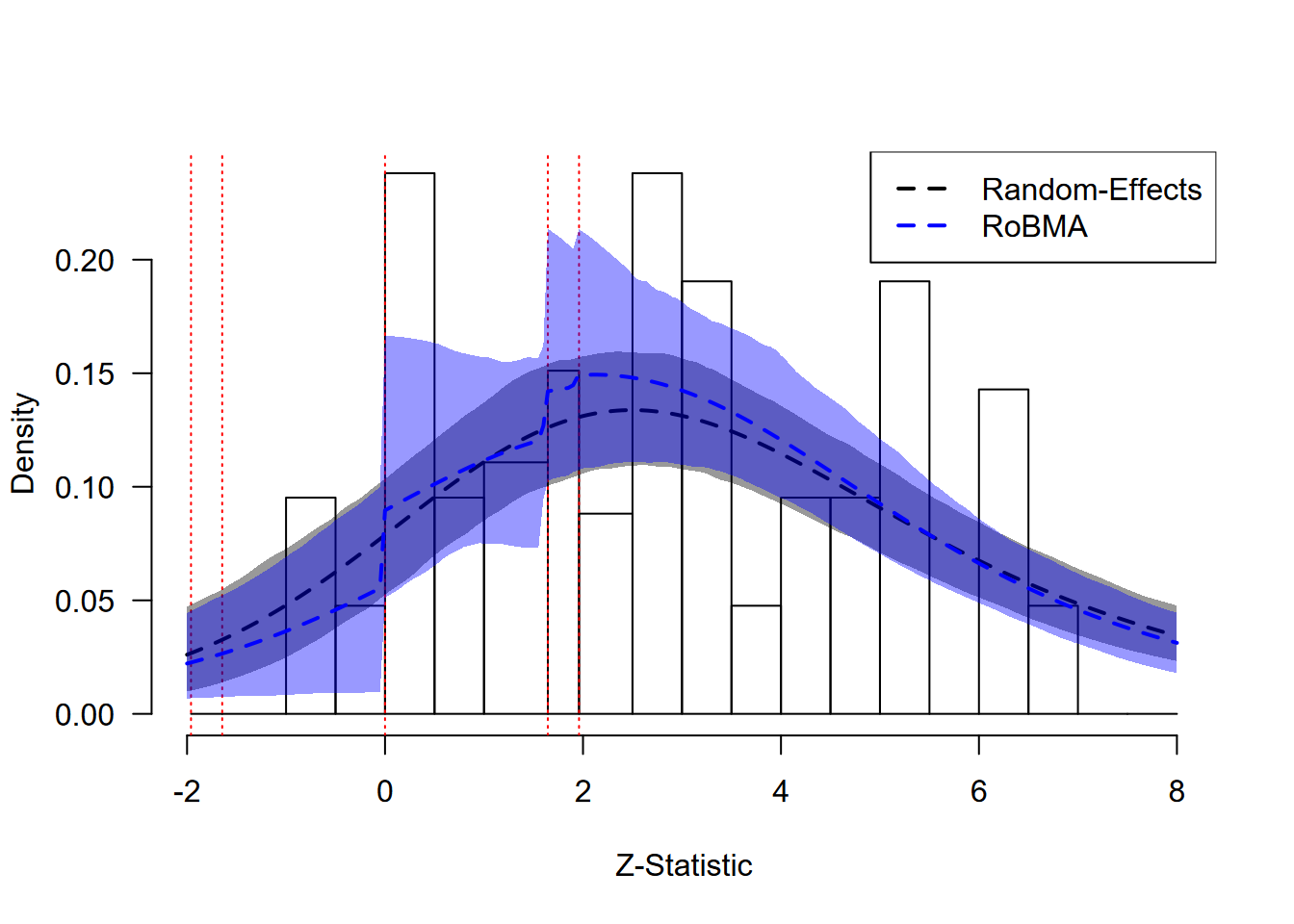
ChatGPT: Model Fit Assessment
Results
The z-curve plot for the ChatGPT data shows a different pattern than the extreme publication bias observed in the social comparison example. While we do not see strong selection at conventional significance thresholds, there is a moderate discontinuity at the transition to non-conforming results (z = 0), suggesting some degree of selection against negative findings.
The random-effects model (black dashed line) provides a better fit to
the data than in the previous example;
however, RoBMA (blue dashed line) captures the discontinuity at zero
slightly better. This visual pattern corresponds to moderate statistical
evidence for publication bias, highlighting a case where both models
might be considered, though the RoBMA model incorporates the uncertainty
about the best model and provides a more complete account of the data
patterns.
Extrapolation to Pre-Publication Bias
We can examine the extrapolation to assess the impact of publication bias:
# Examine extrapolation
plot(zcurve_RoBMA_Wang2025, from = -2, to = 8)
#> 3 z-statistics are out of the plotting range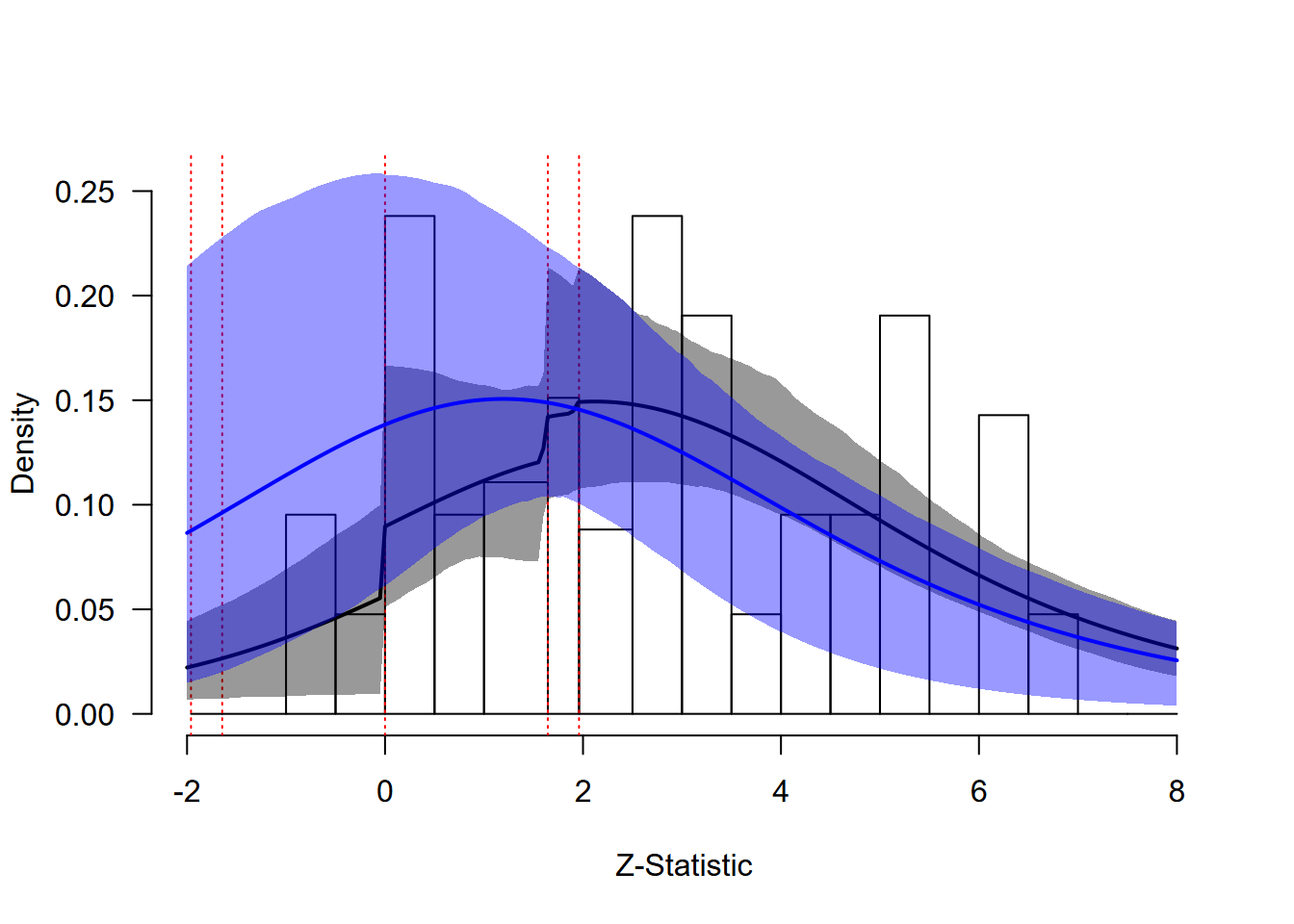
ChatGPT: Extrapolation Analysis
The extrapolated distribution (blue line) shows a more modest difference between the fitted and extrapolated distributions compared to the extreme bias example, reflecting the moderate degree of publication bias in this literature.
Model Results Summary
To quantify these visual patterns, we examine the model summaries:
summary(fit_RE_Wang2025)
#> Call:
#> RoBMA(d = d, r = r, logOR = logOR, OR = OR, z = z, y = y, se = se,
#>     v = v, n = n, lCI = lCI, uCI = uCI, t = t, study_names = study_names,
#>     study_ids = study_ids, data = data, transformation = transformation,
#>     prior_scale = prior_scale, effect_direction = "positive",
#>     model_type = model_type, priors_effect = priors_effect, priors_heterogeneity = priors_heterogeneity,
#>     priors_bias = NULL, priors_effect_null = priors_effect_null,
#>     priors_heterogeneity_null = priors_heterogeneity_null, priors_bias_null = prior_none(),
#>     priors_hierarchical = priors_hierarchical, priors_hierarchical_null = priors_hierarchical_null,
#>     algorithm = algorithm, chains = chains, sample = sample,
#>     burnin = burnin, adapt = adapt, thin = thin, parallel = parallel,
#>     autofit = autofit, autofit_control = autofit_control, convergence_checks = convergence_checks,
#>     save = save, seed = seed, silent = silent)
#>
#> Bayesian model-averaged meta-analysis (normal-normal model)
#> Components summary:
#>               Prior prob. Post. prob. Inclusion BF
#> Effect              1.000       1.000          Inf
#> Heterogeneity       1.000       1.000          Inf
#>
#> Model-averaged estimates:
#>      Mean Median 0.025 0.975
#> mu  0.788  0.788 0.568 1.009
#> tau 0.667  0.659 0.512 0.867
#> The estimates are summarized on the Cohen's d scale (priors were specified on the Cohen's d scale).
#> (Estimated publication weights omega correspond to one-sided p-values.)
summary(fit_RoBMA_Wang2025)
#> Call:
#> RoBMA(d = Wang2025$g, se = Wang2025$se, algorithm = "ss", chains = 5,
#>     sample = 10000, burnin = 5000, adapt = 5000, parallel = TRUE,
#>     save = "min", seed = 1)
#>
#> Robust Bayesian meta-analysis
#> Components summary:
#>               Prior prob. Post. prob. Inclusion BF
#> Effect              0.500       0.669        2.019
#> Heterogeneity       0.500       1.000          Inf
#> Bias                0.500       0.761        3.189
#>
#> Model-averaged estimates:
#>                    Mean Median  0.025 0.975
#> mu                0.380  0.422 -0.042 0.935
#> tau               0.750  0.703  0.506 1.165
#> omega[0,0.025]    1.000  1.000  1.000 1.000
#> omega[0.025,0.05] 0.972  1.000  0.684 1.000
#> omega[0.05,0.5]   0.872  1.000  0.376 1.000
#> omega[0.5,0.95]   0.693  1.000  0.038 1.000
#> omega[0.95,0.975] 0.693  1.000  0.038 1.000
#> omega[0.975,1]    0.694  1.000  0.038 1.000
#> PET               0.647  0.000  0.000 3.345
#> PEESE             0.194  0.000  0.000 3.177
#> The estimates are summarized on the Cohen's d scale (priors were specified on the Cohen's d scale).
#> (Estimated publication weights omega correspond to one-sided p-values.)
The random-effects model yields an effect size estimate of g = 0.79 [0.57, 1.01], while the RoBMA model accounting for selection produces a more conservative g = 0.38 [-0.04, 0.94]. Importantly, the results show an extreme degree of between-study heterogeneity, tau = 0.75 [0.51, 1.17], that greatly complicates feasible implications and recommendations. This demonstrates the moderate nature of the publication bias, where the adjusted estimate is meaningfully smaller but not completely reduced. The Bayes factor for publication bias (BF_bias = 3.2) provides moderate evidence for publication bias, and the evidence for the effect becomes weak (BF_effect = 2).
Z-Curve Summary Metrics
This moderate publication bias pattern is reflected in the summary statistics,
# Extract z-curve summary metrics for ChatGPT data
summary(zcurve_RoBMA_Wang2025)
#> Call:
#> as_zcurve: RoBMA(d = Wang2025$g, se = Wang2025$se, algorithm = "ss", chains = 5,
#>     sample = 10000, burnin = 5000, adapt = 5000, parallel = TRUE,
#>     save = "min", seed = 1)
#>
#> Z-curve
#> Model-averaged estimates:
#>             Mean Median 0.025  0.975
#> EDR        0.607  0.619 0.433  0.740
#> Soric FDR  0.036  0.032 0.018  0.069
#> Missing N 13.652  0.000 0.000 57.926
#> Estimated using 42 estimates, 27 significant (ODR = 0.64, 95 CI [0.48, 0.78]).
which show a moderate-to-high EDR of 0.61 and around 14 missing estimates.
Example 4: Framing Effects from Many Labs 2
Our final example analyzes registered replication reports of the classic framing effect on decision making (Tversky & Kahneman, 1981) conducted as part of the Many Labs 2 project (Klein et al., 2018). This dataset provides an ideal test case for z-curve diagnostics because the pre-registered nature of these studies does not allow for publication bias. The analysis includes 55 effect size estimates that examine how framing influences decision-making preferences.
Data Analysis and Model Fitting
# Load the Many Labs 2 framing effect data
data("ManyLabs16", package = "RoBMA")
head(ManyLabs16)
#>           y        se
#> 1 0.3507108 0.2198890
#> 2 0.1238568 0.1496303
#> 3 0.1752287 0.3055819
#> 4 0.5125227 0.2012544
#> 5 0.4573484 0.1505897
#> 6 0.6846411 0.1870689
# Fit models and create z-curve objects
fit_RE_ManyLabs16 <- NoBMA(d = ManyLabs16$y, se = ManyLabs16$se,
                           priors_effect_null = NULL, priors_heterogeneity_null = NULL,
                           algorithm = "ss", sample = 10000, burnin = 5000, adapt = 5000,
                           chains = 5, parallel = TRUE, seed = 1)
fit_RoBMA_ManyLabs16 <- RoBMA(d = ManyLabs16$y, se = ManyLabs16$se,
                              algorithm = "ss", sample = 10000, burnin = 5000, adapt = 5000,
                              chains = 5, parallel = TRUE, seed = 1)

zcurve_RE_ManyLabs16    <- as_zcurve(fit_RE_ManyLabs16)
zcurve_RoBMA_ManyLabs16 <- as_zcurve(fit_RoBMA_ManyLabs16)
Z-Curve Assessment
# Assess model fit - should show good agreement
hist(zcurve_RoBMA_ManyLabs16)
#> 2 z-statistics are out of the plotting range
lines(zcurve_RE_ManyLabs16, col = "black", lty = 2, lwd = 2)
lines(zcurve_RoBMA_ManyLabs16, col = "blue", lty = 2, lwd = 2)
legend("topleft",
       legend = c("Random-Effects", "RoBMA"),
       col = c("black", "blue"),
       lty = 2, lwd = 2)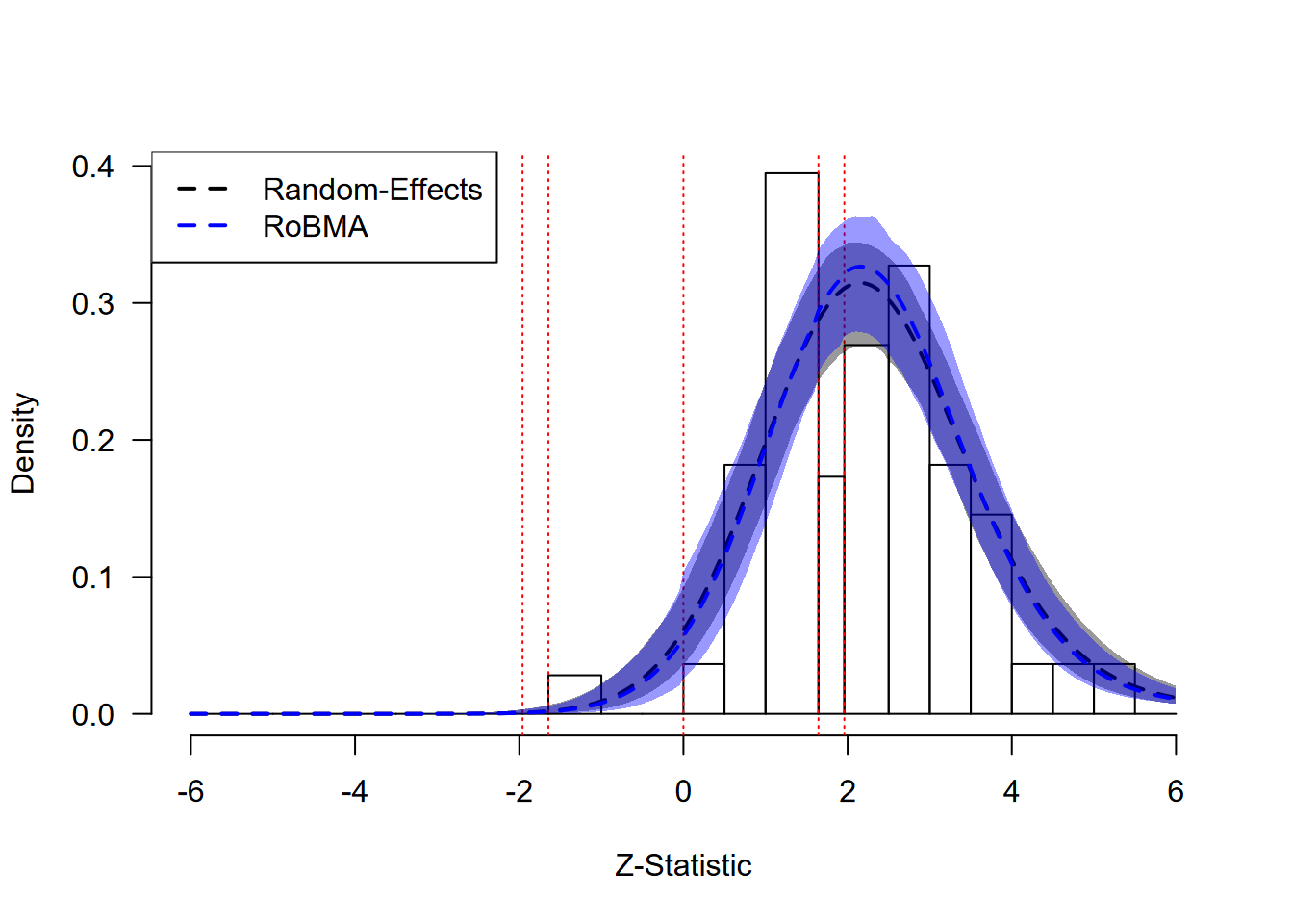
Framing Effects: Model Fit Assessment
Results
The z-curve plot for the Many Labs 2 framing effects demonstrates what we expect to see in the absence of publication bias. The observed distribution of z-statistics (gray bars) appears smooth without sharp discontinuities at significance thresholds or at zero. Both the random-effects model (black dashed line) and RoBMA (blue dashed line) provide essentially identical fits to the data, with their posterior predictive distributions overlapping almost perfectly.
This close agreement between models indicates that either approach would be appropriate for these data. The absence of publication bias is further confirmed by the statistical evidence: RoBMA provides moderate evidence against publication bias, demonstrating how the method appropriately penalizes unnecessary model complexity when simpler models explain the data equally well.
Extrapolation to Pre-Publication Bias
We can examine whether there would be any difference in the absence of publication bias:
# Extrapolation should show minimal change
plot(zcurve_RoBMA_ManyLabs16)
#> 2 z-statistics are out of the plotting range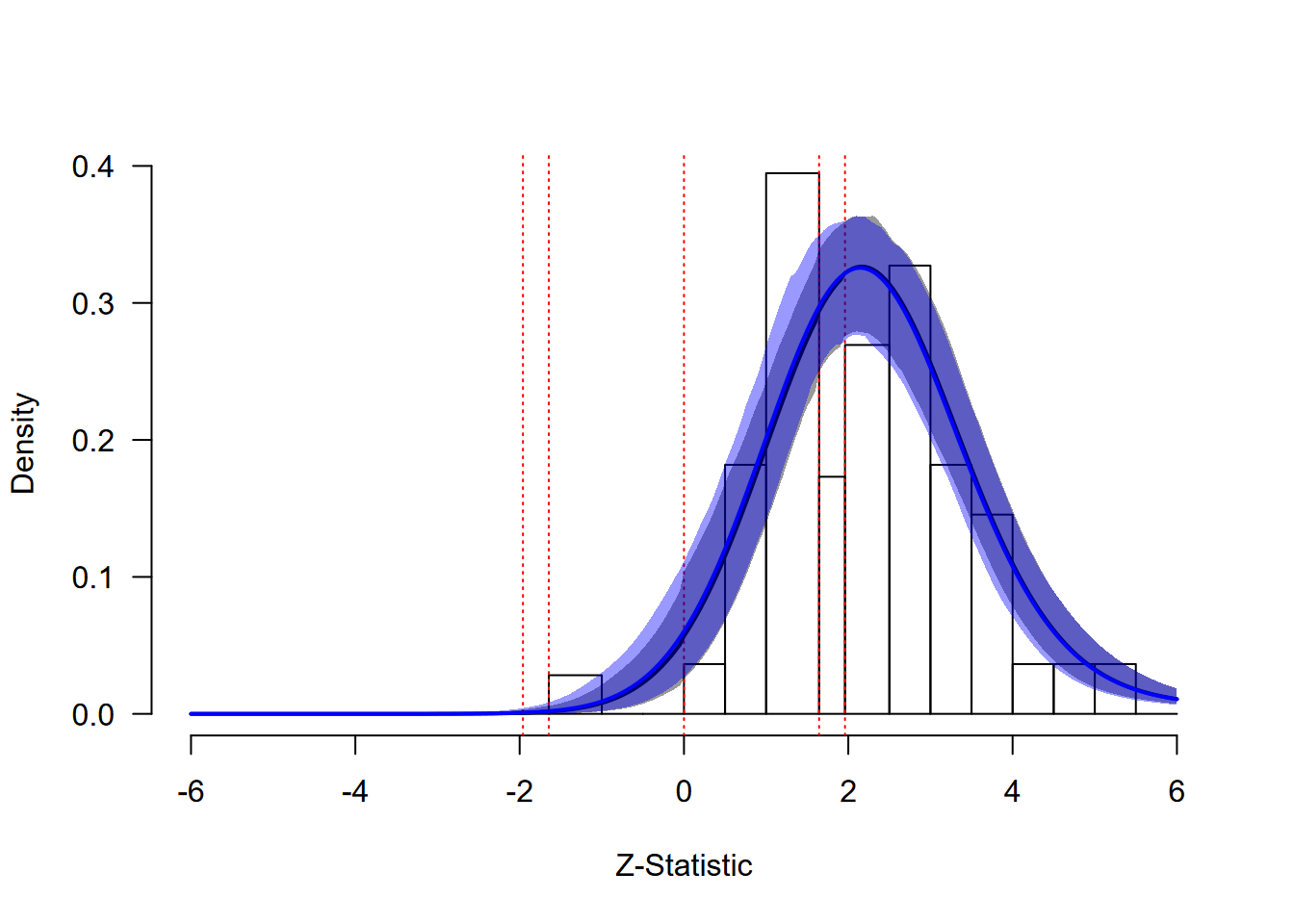
Framing Effects: Extrapolation Analysis
The extrapolated distribution (blue line) shows virtually no difference between the fitted and extrapolated distributions, confirming that publication bias has minimal impact in this well-designed replication project. This example illustrates the ideal scenario where traditional meta-analytic approaches are fully justified.
Model Results Summary
The quantitative results confirm the visual impression:
Both models yield virtually identical effect size estimate of d = 0.43 [0.35, 0.49]. The Bayes factor for publication bias (BF_bias = 0.21) provides moderate evidence against the presence of publication bias, appropriately penalizing the more complex model when it offers no advantage. This demonstrates the method’s ability to distinguish between necessary and unnecessary model complexity.
Z-Curve Summary Metrics
The absence of publication bias is reflected in the publication bias assessment statistics — a moderate EDR matching the ODR and no missing studies.
# Extract z-curve summary metrics for Many Labs 2 data
summary(zcurve_RoBMA_ManyLabs16)
#> Call:
#> as_zcurve: RoBMA(d = ManyLabs16$y, se = ManyLabs16$se, algorithm = "ss",
#>     chains = 5, sample = 10000, burnin = 5000, adapt = 5000,
#>     parallel = TRUE, save = "min", seed = 1)
#>
#> Z-curve
#> Model-averaged estimates:
#>            Mean Median 0.025 0.975
#> EDR       0.587  0.596 0.452 0.675
#> Soric FDR 0.038  0.036 0.025 0.064
#> Missing N 0.344  0.000 0.000 4.289
#> Estimated using 55 estimates, 31 significant (ODR = 0.56, 95 CI [0.42, 0.69]).
Conclusions
Z-curve plots are an intuitive diagnostic tool for assessing publication bias and model fit (Bartoš & Schimmack, 2025). By visualizing the distribution of test statistics and comparing observed patterns with model-implied expectations, researchers can make more informed decisions about their analytic approach using the RoBMA package (Bartoš & Maier, 2020).
Z-curve diagnostics are particularly informative when applied to moderate to large meta-analyses (typically >20-30 studies), where histogram patterns become interpretable. Publication bias and QRP might produce similar patterns of results. The z-curve diagnostics cannot distinguish between them; however, it might help in assessing whether the model approximates the observed data well. They are especially useful for model comparison scenarios when they provide a visual supplement to statistical tests like inclusion Bayes factors.
The following points are important for interpreting z-curve diagnostics:
- Sharp drops in the observed distribution at z = 0, z = ±1.64, or z = ±1.96 suggest publication bias.
- Models whose posterior predictive distributions closely match the observed pattern should be preferred.
- Large differences between fitted and extrapolated distributions indicate substantial publication bias.
- Visual assessment should complement formal statistical tests.