Informed Bayesian Model-Averaged Meta-Analysis in Medicine

František Bartoš

2024-12-12

Bayesian model-averaged meta-analysis allows researchers to seamlessly incorporate available prior information into the analysis (Bartoš et al., 2021; Gronau et al., 2017, 2021). This vignette illustrates how to do this with an example from Bartoš et al. (2021), who developed informed prior distributions for meta-analyses of continuous outcomes based on the Cochrane database of systematic reviews. Then, we extend the example by incorporating publication bias adjustment with robust Bayesian meta-analysis (Bartoš et al., 2023; Maier et al., 2023).

Reproducing Informed Bayesian Model-Averaged Meta-Analysis (BMA)

We illustrate how to fit the informed BMA (not adjusting for publication bias) using the RoBMA R package. For this purpose, we reproduce the dentine hypersensitivity example from Bartoš et al. (2021), who reanalyzed five studies with a tactile outcome assessment that were subjected to a meta-analysis by Poulsen et al. (2006).

We load the dentine hypersensitivity data included in the package.

library(RoBMA)

data("Poulsen2006", package = "RoBMA")
Poulsen2006
#>           d        se               study
#> 1 0.9073050 0.2720456     STD-Schiff-1994
#> 2 0.7207589 0.1977769  STD-Silverman-1996
#> 3 1.3305829 0.2721648   STD-Sowinski-2000
#> 4 1.7688872 0.2656483 STD-Schiff-2000-(2)
#> 5 1.3286828 0.3582617     STD-Schiff-1998

To reproduce the analysis from the example, we need to set informed empirical prior distributions for the effect sizes ($\mu$) and heterogeneity ($\tau$) parameters that Bartoš et al. (2021) obtained from the Cochrane database of systematic reviews. We can either set them manually,

fit_BMA <- RoBMA(d = Poulsen2006$d, se = Poulsen2006$se, study_names = Poulsen2006$study,
                 priors_effect        = prior(distribution = "t", parameters = list(location = 0, scale = 0.51, df = 5)),
                 priors_heterogeneity = prior(distribution = "invgamma", parameters = list(shape = 1.79, scale = 0.28)),
                 priors_bias          = NULL,
                 transformation = "cohens_d", seed = 1, parallel = TRUE)

with priors_effect and priors_heterogeneity corresponding to the $\delta \sim T(0,0.51,5)$ and $\tau \sim InvGamma(1.79,0.28)$ informed prior distributions for the “oral health” subfield and removing the publication bias adjustment models by setting priors_bias = NULL$^1$. Note that the package contains function NoBMA() from version 3.1 which skips publication bias adjustment directly.

Alternatively, we can utilize the prior_informed function that prepares informed prior distributions for the individual medical subfields automatically.

fit_BMA <- RoBMA(d = Poulsen2006$d, se = Poulsen2006$se, study_names = Poulsen2006$study,
                 priors_effect        = prior_informed(name = "oral health", parameter = "effect", type = "smd"),
                 priors_heterogeneity = prior_informed(name = "oral health", parameter = "heterogeneity", type = "smd"),
                 priors_bias          = NULL,
                 transformation = "cohens_d", seed = 1, parallel = TRUE)

The name argument specifies the medical subfield name (use print(BayesTools::prior_informed_medicine_names) to check names of all available subfields). The parameter argument specifies whether we want prior distribution for the effect size or heterogeneity. Finally, the type argument specifies what type of measure we use for the meta-analysis (see ?prior_informed for more details regarding the informed prior distributions).

We obtain the output with the summary function. Adding the conditional = TRUE argument allows us to inspect the conditional estimates, i.e., the effect size estimate assuming that the models specifying the presence of the effect are true and the heterogeneity estimates assuming that the models specifying the presence of heterogeneity are true$^2$.

summary(fit_BMA, conditional = TRUE)
#> Call:
#> RoBMA(d = Poulsen2006$d, se = Poulsen2006$se, study_names = Poulsen2006$study, 
#>     transformation = "cohens_d", priors_effect = prior_informed(name = "oral health", 
#>         parameter = "effect", type = "smd"), priors_heterogeneity = prior_informed(name = "oral health", 
#>         parameter = "heterogeneity", type = "smd"), priors_bias = NULL, 
#>     parallel = TRUE, seed = 1)
#> 
#> Robust Bayesian meta-analysis
#> Components summary:
#>               Models Prior prob. Post. prob. Inclusion BF
#> Effect           2/4       0.500       0.995      217.517
#> Heterogeneity    2/4       0.500       0.778        3.511
#> 
#> Model-averaged estimates:
#>      Mean Median 0.025 0.975
#> mu  1.076  1.088 0.664 1.422
#> tau 0.231  0.208 0.000 0.726
#> The estimates are summarized on the Cohen's d scale (priors were specified on the Cohen's d scale).
#> 
#> Conditional estimates:
#>      Mean Median 0.025 0.975
#> mu  1.082  1.090 0.701 1.422
#> tau 0.297  0.255 0.075 0.779
#> The estimates are summarized on the Cohen's d scale (priors were specified on the Cohen's d scale).

The output from the summary.RoBMA() function has 3 parts. The first one under the ‘Robust Bayesian Meta-Analysis’ heading provides a basic summary of the fitted models by component types (presence of the Effect and Heterogeneity). The table summarizes the prior and posterior probabilities and the inclusion Bayes factors of the individual components. The results show that the inclusion Bayes factor for the effect corresponds to the one reported in Bartoš et al. (2021), $\text{BF}_{10} = 218.53$ and $\text{BF}_{\text{rf}} = 3.52$ (up to an MCMC error).

The second part under the ‘Model-averaged estimates’ heading displays the parameter estimates model-averaged across all specified models (i.e., including models specifying the effect size to be zero). We ignore this section and move to the last part.

The third part under the ‘Conditional estimates’ heading displays the conditional effect size estimate corresponding to the one reported in Bartoš et al. (2021), $\delta = 1.082$, 95% CI [0.686,1.412], and a heterogeneity estimate (not reported previously).

Visualizing the Results

The RoBMA package provides extensive options for visualizing the results. Here, we visualize the prior (grey) and posterior (black) distribution for the mean parameter.

plot(fit_BMA, parameter = "mu", prior = TRUE)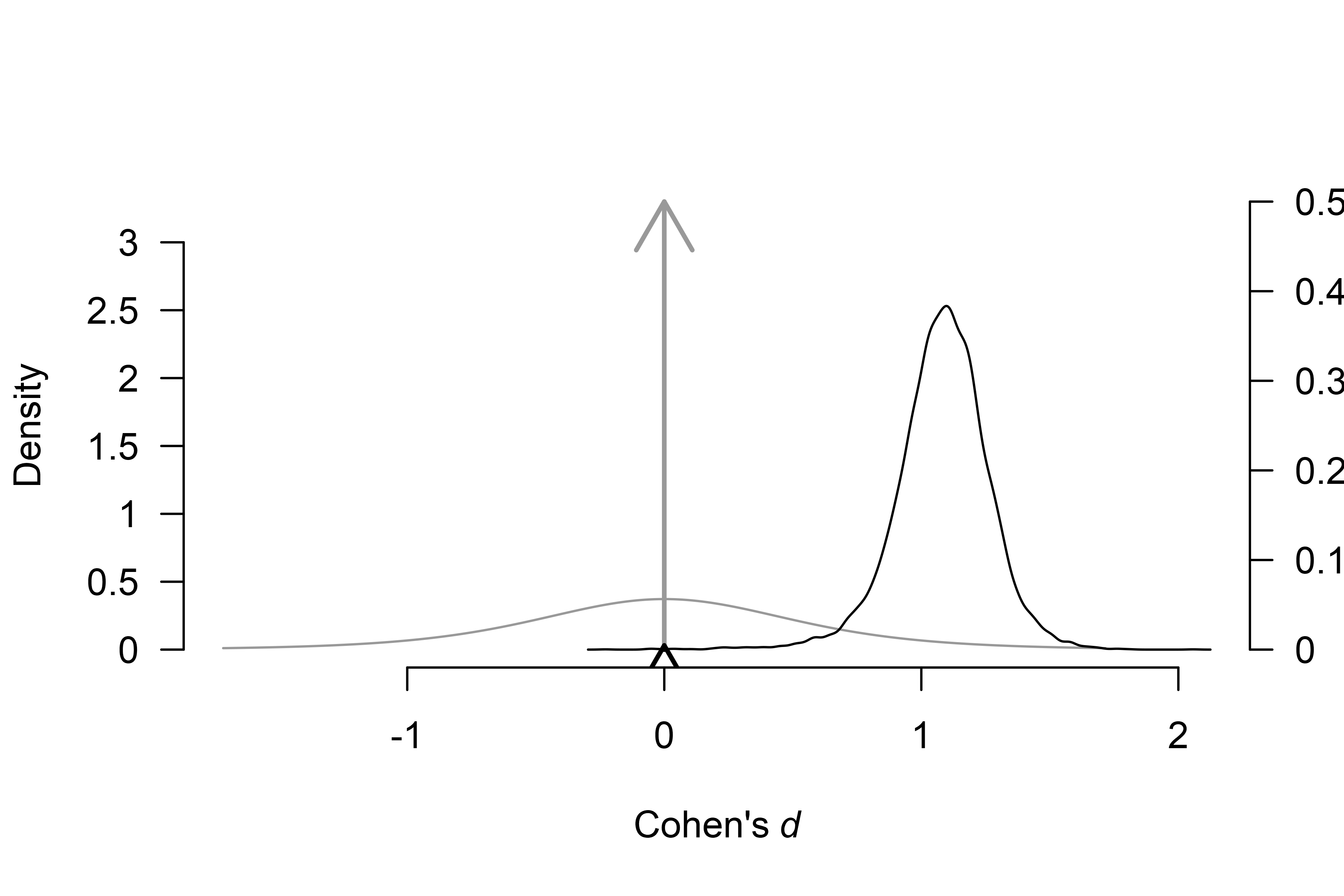

By default, the function plots the model-averaged estimates across all models; the arrows represent the probability of a spike, and the lines represent the posterior density under models assuming non-zero effect. The secondary y-axis (right) shows the probability of the spike (at value 0) decreasing from 0.50, to 0.005 (also obtainable from the ‘Robust Bayesian Meta-Analysis’ field in summary.RoBMA() function).

To visualize the conditional effect size estimate, we can add the conditional = TRUE argument,

plot(fit_BMA, parameter = "mu", prior = TRUE, conditional = TRUE)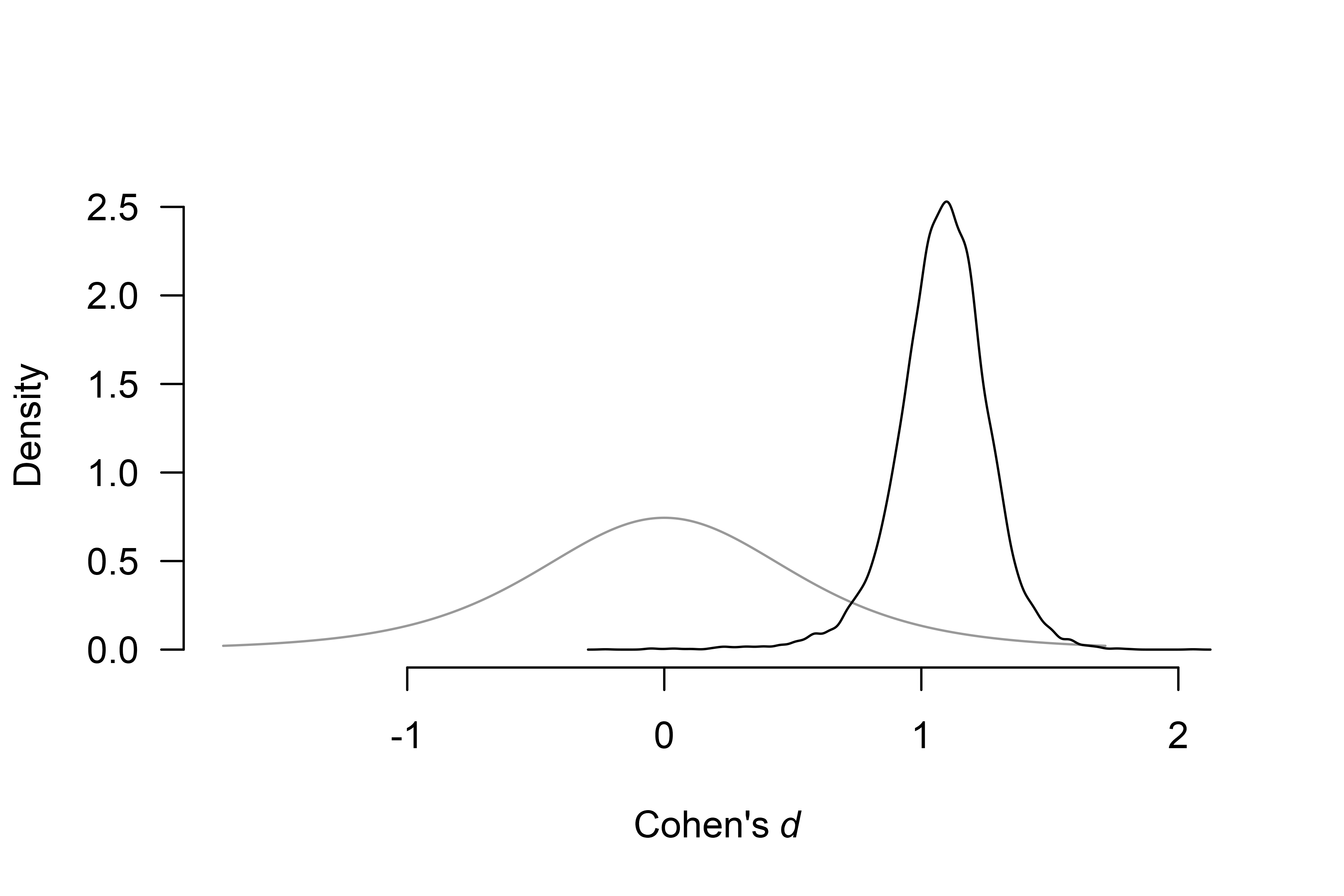

which displays only the model-averaged posterior distribution of the effect size parameter for models assuming the presence of the effect.

We can also visualize the estimates from the individual models used in the ensemble. We do that with the plot_models() function, which visualizes the effect size estimates and 95% CI of each specified model included in the ensemble. Model 1 corresponds to the fixed effect model assuming the absence of the effect, $H_0^{\text{f}}$, Model 2 corresponds to the random effect model assuming the absence of the effect, $H_0^{\text{r}}$, Model 3 corresponds to the fixed effect model assuming the presence of the effect, $H_1^{\text{f}}$, and Model 4 corresponds to the random effect model assuming the presence of the effect, $H_1^{\text{r}}$). The size of the square representing the mean estimate reflects the posterior model probability of the model, which is also displayed in the right-hand side panel. The bottom part of the figure shows the model averaged-estimate that is a combination of the individual model posterior distributions weighted by the posterior model probabilities.

plot_models(fit_BMA)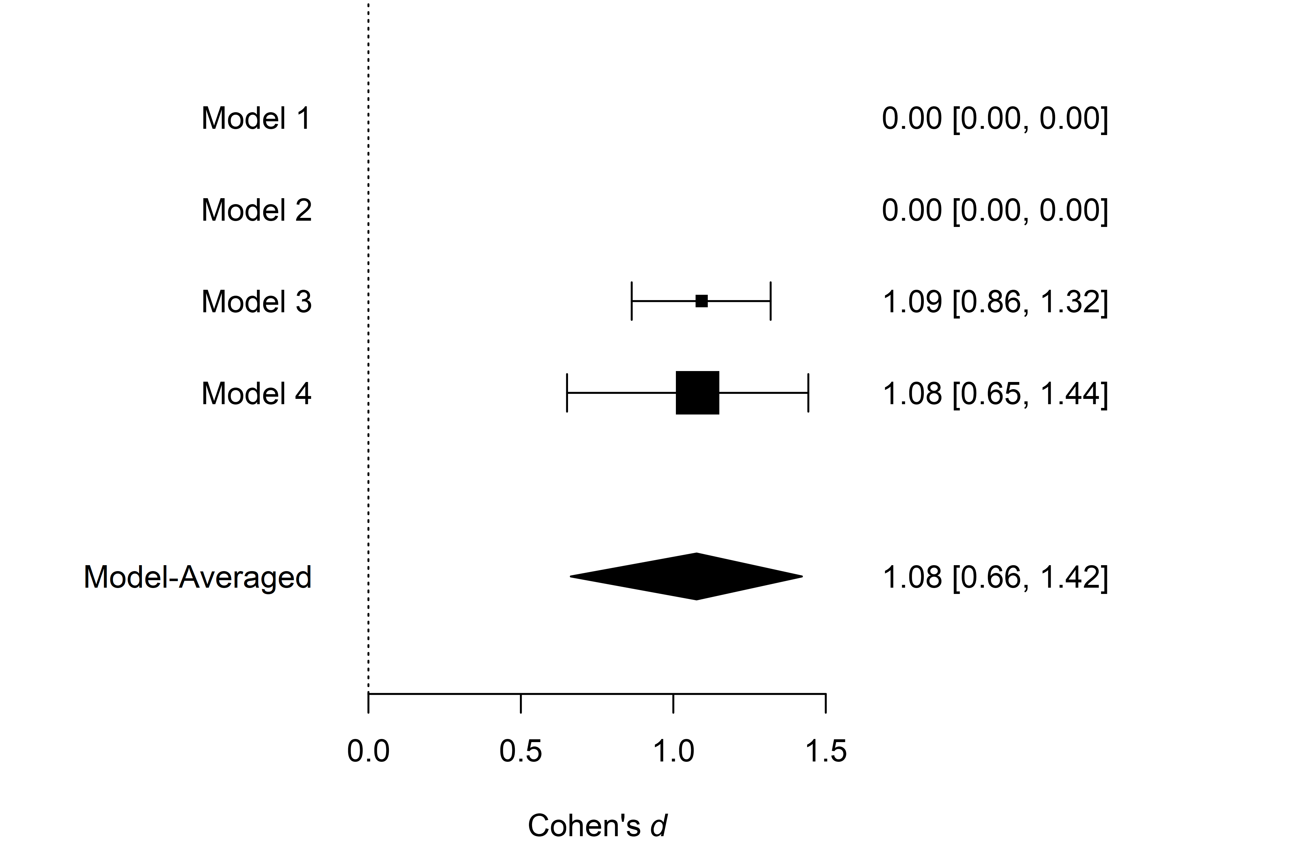

We see that the posterior model probability of the first two models decreased to essentially zero (when rounding to two decimals), completely omitting their estimates from the figure. Furthermore, the much larger box of Model 4 (the random effect model assuming the presence of the effect) shows that Model 4 received the largest share of the posterior probability, $P(H_1^{\text{r}}) = 0.77$)

The last type of visualization that we show here is the forest plot. It displays the original studies’ effects and the meta-analytic estimate within one figure. It can be requested by using the forest() function. Here, we again set the conditional = TRUE argument to display the conditional model-averaged effect size estimate at the bottom.

forest(fit_BMA, conditional = TRUE)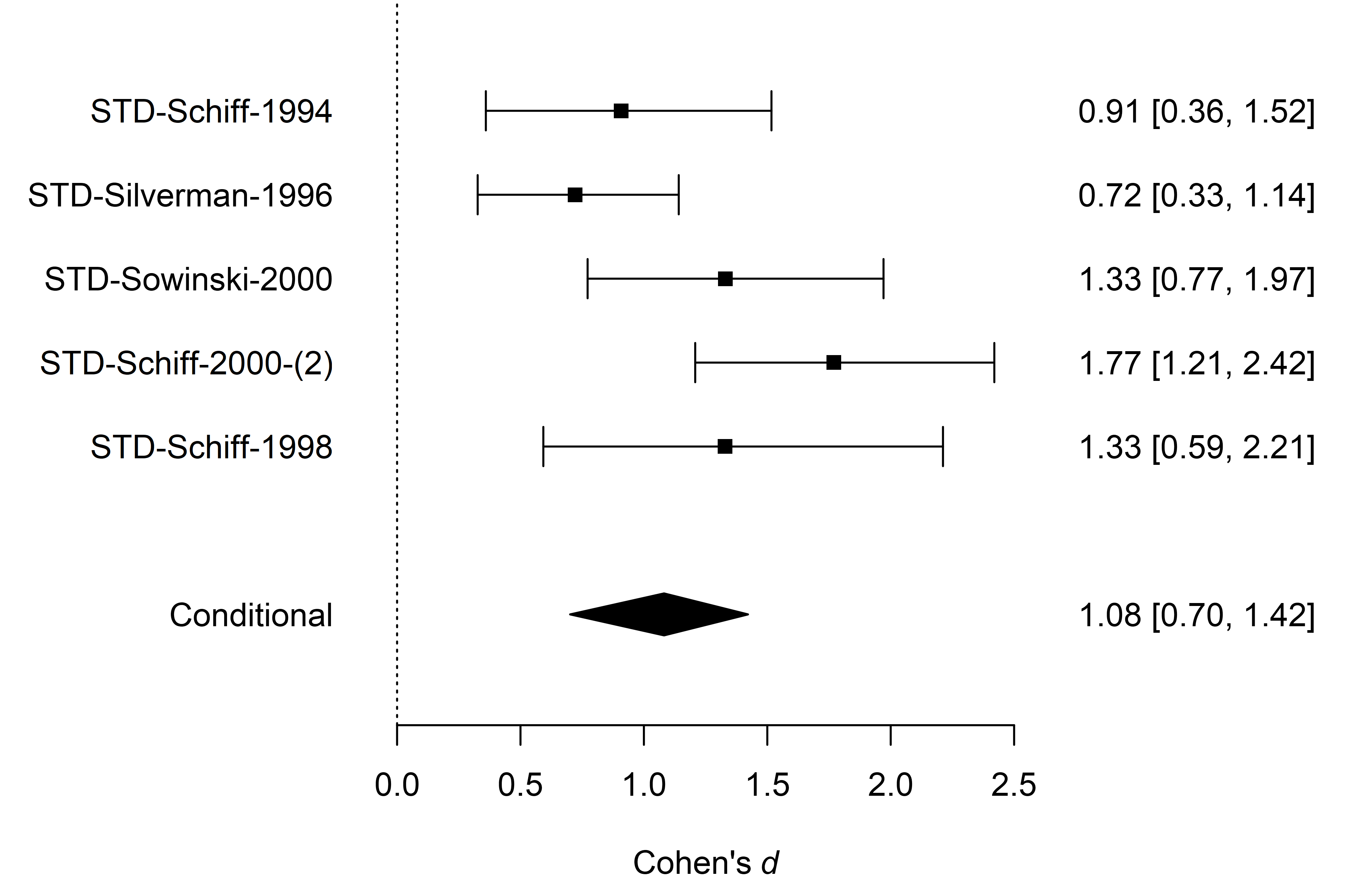

For more options provided by the plotting function, see its documentation by using ?plot.RoBMA(), ?plot_models(), and ?forest().

Adjusting for Publication Bias with Robust Bayesian Meta-Analysis

Finally, we illustrate how to adjust our informed BMA for publication bias with robust Bayesian meta-analysis Maier et al. (2023). In short, we specify additional models assuming the presence of the publication bias and correcting for it by either specifying a selection model operating on $p$-values (Vevea & Hedges, 1995) or by specifying a publication bias adjustment method correcting for the relationship between effect sizes and standard errors – PET-PEESE (Stanley, 2017; Stanley & Doucouliagos, 2014). See Bartoš et al. (2022) for a tutorial.

To obtain a proper before and after publication bias adjustment comparison, we fit the informed BMA model but using the default effect size transformation (Fisher’s $z$).

fit_BMAb <- RoBMA(d = Poulsen2006$d, se = Poulsen2006$se, study_names = Poulsen2006$study,
                  priors_effect        = prior_informed(name = "oral health", parameter = "effect", type = "smd"),
                  priors_heterogeneity = prior_informed(name = "oral health", parameter = "heterogeneity", type = "smd"),
                  priors_bias          = NULL,
                  seed = 1, parallel = TRUE)

summary(fit_BMAb, conditional = TRUE)
#> Call:
#> RoBMA(d = Poulsen2006$d, se = Poulsen2006$se, study_names = Poulsen2006$study, 
#>     priors_effect = prior_informed(name = "oral health", parameter = "effect", 
#>         type = "smd"), priors_heterogeneity = prior_informed(name = "oral health", 
#>         parameter = "heterogeneity", type = "smd"), priors_bias = NULL, 
#>     parallel = TRUE, seed = 1)
#> 
#> Robust Bayesian meta-analysis
#> Components summary:
#>               Models Prior prob. Post. prob. Inclusion BF
#> Effect           2/4       0.500       0.997      347.932
#> Heterogeneity    2/4       0.500       0.723        2.608
#> 
#> Model-averaged estimates:
#>      Mean Median 0.025 0.975
#> mu  1.045  1.052 0.705 1.344
#> tau 0.186  0.163 0.000 0.623
#> The estimates are summarized on the Cohen's d scale (priors were specified on the Cohen's d scale).
#> 
#> Conditional estimates:
#>      Mean Median 0.025 0.975
#> mu  1.048  1.053 0.720 1.344
#> tau 0.256  0.220 0.064 0.681
#> The estimates are summarized on the Cohen's d scale (priors were specified on the Cohen's d scale).

We obtain noticeably stronger evidence for the presence of the effect. This is a result of placing more weights on the fixed-effect models, especially the fixed-effect model assuming the presence of the effect $H_1^f$. In our case, the increase in the posterior model probability of $H_1^f$ occurred because this model predicted the data slightly better after removing the correlation between effect sizes and standard errors (a consequence of using Fisher’s $z$ transformation). Nevertheless, the conditional effect size estimate stayed almost the same.

Now, we fit the publication bias-adjusted model by simply removing the priors_bias = NULL argument, which allows us to obtain the default 36 models ensemble called RoBMA-PSMA (Bartoš et al., 2023).

fit_RoBMA <- RoBMA(d = Poulsen2006$d, se = Poulsen2006$se, study_names = Poulsen2006$study,
                   priors_effect        = prior_informed(name = "oral health", parameter = "effect", type = "smd"),
                   priors_heterogeneity = prior_informed(name = "oral health", parameter = "heterogeneity", type = "smd"),
                   seed = 1, parallel = TRUE)

summary(fit_RoBMA, conditional = TRUE)
#> Call:
#> RoBMA(d = Poulsen2006$d, se = Poulsen2006$se, study_names = Poulsen2006$study, 
#>     priors_effect = prior_informed(name = "oral health", parameter = "effect", 
#>         type = "smd"), priors_heterogeneity = prior_informed(name = "oral health", 
#>         parameter = "heterogeneity", type = "smd"), parallel = TRUE, 
#>     seed = 1)
#> 
#> Robust Bayesian meta-analysis
#> Components summary:
#>               Models Prior prob. Post. prob. Inclusion BF
#> Effect         18/36       0.500       0.858        6.022
#> Heterogeneity  18/36       0.500       0.714        2.502
#> Bias           32/36       0.500       0.697        2.304
#> 
#> Model-averaged estimates:
#>                    Mean Median 0.025  0.975
#> mu                0.722  0.880 0.000  1.283
#> tau               0.202  0.161 0.000  0.799
#> omega[0,0.025]    1.000  1.000 1.000  1.000
#> omega[0.025,0.05] 0.943  1.000 0.329  1.000
#> omega[0.05,0.5]   0.874  1.000 0.071  1.000
#> omega[0.5,0.95]   0.855  1.000 0.042  1.000
#> omega[0.95,0.975] 0.866  1.000 0.050  1.000
#> omega[0.975,1]    0.897  1.000 0.057  1.000
#> PET               0.931  0.000 0.000  4.927
#> PEESE             1.131  0.000 0.000 12.261
#> The estimates are summarized on the Cohen's d scale (priors were specified on the Cohen's d scale).
#> (Estimated publication weights omega correspond to one-sided p-values.)
#> 
#> Conditional estimates:
#>                    Mean Median  0.025  0.975
#> mu                0.838  0.938 -0.035  1.297
#> tau               0.285  0.227  0.064  0.906
#> omega[0,0.025]    1.000  1.000  1.000  1.000
#> omega[0.025,0.05] 0.736  0.829  0.092  1.000
#> omega[0.05,0.5]   0.411  0.373  0.014  0.951
#> omega[0.5,0.95]   0.320  0.249  0.008  0.919
#> omega[0.95,0.975] 0.376  0.311  0.009  0.958
#> omega[0.975,1]    0.518  0.425  0.010  1.000
#> PET               2.909  3.136  0.171  5.614
#> PEESE             7.048  6.034  0.375 18.162
#> The estimates are summarized on the Cohen's d scale (priors were specified on the Cohen's d scale).
#> (Estimated publication weights omega correspond to one-sided p-values.)

We notice the additional values in the ‘Components summary’ table in the ‘Bias’ row. The model is now extended with 32 publication bias adjustment models that account for 50% of the prior model probability. When comparing the RoBMA to the second BMA fit, we notice a large decrease in the inclusion Bayes factor for the presence of the effect $\text{BF}_{10} = 6.02$ vs. $\text{BF}_{10} = 347.93$, which still, however, presents moderate evidence for the presence of the effect. We can further quantify the evidence in favor of the publication bias with the inclusion Bayes factor for publication bias $\text{BF}_{pb} = 2.30$, which can be interpreted as weak evidence in favor of publication bias.

We can also compare the publication bias unadjusted and publication bias-adjusted conditional effect size estimates. Including models assuming publication bias into our model-averaged estimate (assuming the presence of the effect) slightly decreases the estimated effect to $\delta = 0.838$, 95% CI [-0.035, 1.297] with a much wider confidence interval, as visualized in the prior and posterior conditional effect size estimate plot.

plot(fit_RoBMA, parameter = "mu", prior = TRUE, conditional = TRUE)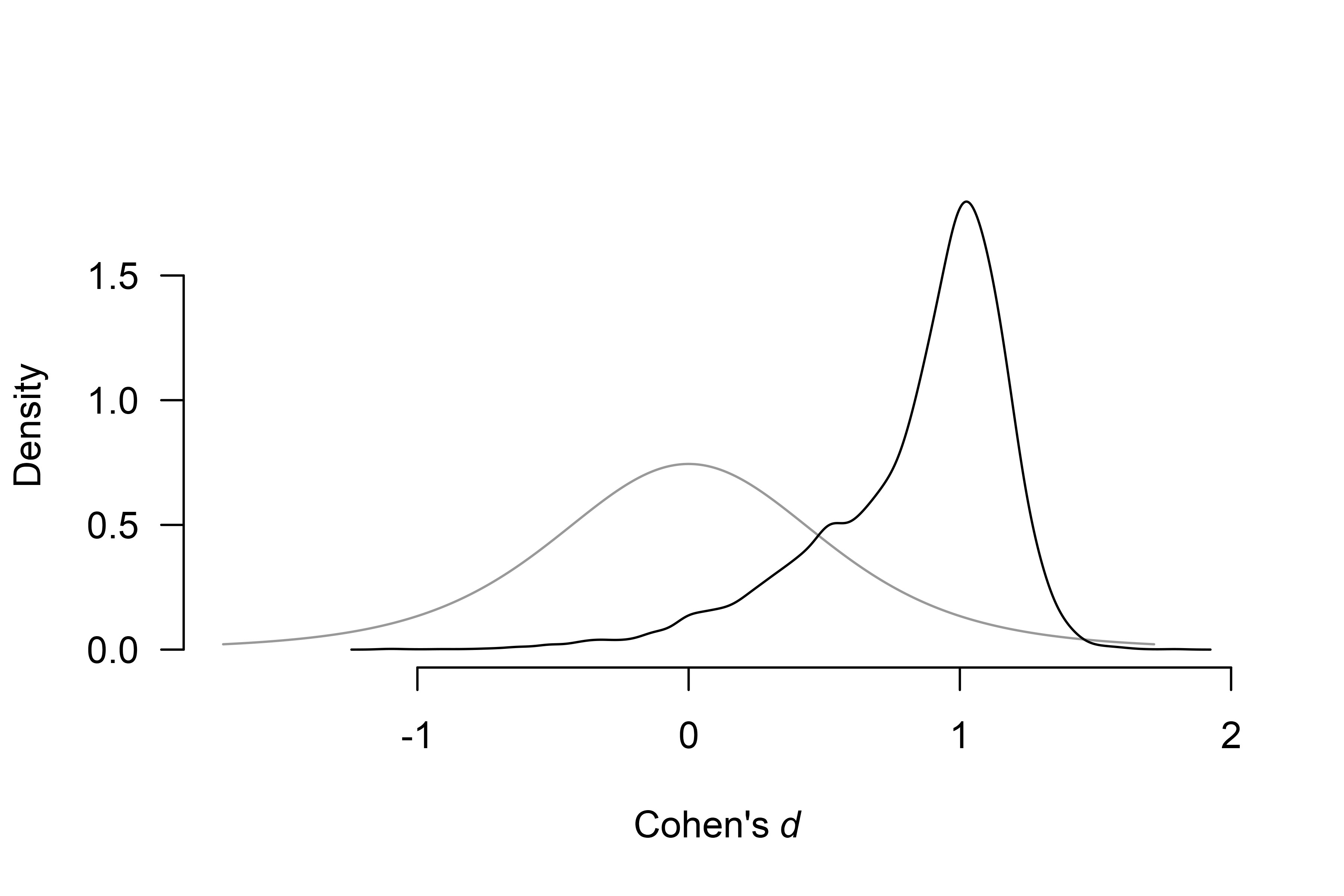

Footnotes

$^1$ The additional setting transformation = "cohens_d" allows us to get more comparable results with the metaBMA R package since RoBMA otherwise internally transforms the effect sizes to Fisher’s $z$ for the fitting purposes. The seed = 1 and parallel = TRUE options grant us exact reproducibility of the results and parallelization of the fitting process.

$^2$ The model-averaged estimates that RoBMA returns by default model-averaged across all specified models – a different behavior from the metaBMA package that by default returns what we call “conditional” estimates in RoBMA.

References

Bartoš, F., Gronau, Q. F., Timmers, B., Otte, W. M., Ly, A., & Wagenmakers, E.-J. (2021). Bayesian model-averaged meta-analysis in medicine. Statistics in Medicine, 40(30), 6743–6761. https://doi.org/10.1002/sim.9170

Bartoš, F., Maier, Maximilian, Quintana, D. S., & Wagenmakers, E.-J. (2022). Adjusting for publication bias in JASP and R — Selection models, PET-PEESE, and robust Bayesian meta-analysis. Advances in Methods and Practices in Psychological Science, 5(3), 1–19. https://doi.org/10.1177/25152459221109259

Bartoš, F., Maier, M., Wagenmakers, E.-J., Doucouliagos, H., & Stanley, T. D. (2023). Robust Bayesian meta-analysis: Model-averaging across complementary publication bias adjustment methods. Research Synthesis Methods, 14(1), 99–116. https://doi.org/10.1002/jrsm.1594

Gronau, Q. F., Heck, D. W., Berkhout, S. W., Haaf, J. M., & Wagenmakers, E.-J. (2021). A primer on Bayesian model-averaged meta-analysis. Advances in Methods and Practices in Psychological Science, 4(3), 1–19. https://doi.org/10.1177/25152459211031256

Gronau, Q. F., Van Erp, S., Heck, D. W., Cesario, J., Jonas, K. J., & Wagenmakers, E.-J. (2017). A Bayesian model-averaged meta-analysis of the power pose effect with informed and default priors: The case of felt power. Comprehensive Results in Social Psychology, 2(1), 123–138. https://doi.org/10.1080/23743603.2017.1326760

Maier, M., Bartoš, F., & Wagenmakers, E.-J. (2023). Robust Bayesian meta-analysis: Addressing publication bias with model-averaging. Psychological Methods, 28(1), 107–122. https://doi.org/10.1037/met0000405

Poulsen, S., Errboe, M., Mevil, Y. L., & Glenny, A.-M. (2006). Potassium containing toothpastes for dentine hypersensitivity. Cochrane Database of Systematic Reviews, 3. https://doi.org/10.1002/14651858.cd001476.pub2

Stanley, T. D. (2017). Limitations of PET-PEESE and other meta-analysis methods. Social Psychological and Personality Science, 8(5), 581–591. https://doi.org/10.1177/1948550617693062

Stanley, T. D., & Doucouliagos, H. (2014). Meta-regression approximations to reduce publication selection bias. Research Synthesis Methods, 5(1), 60–78. https://doi.org/10.1002/jrsm.1095

Vevea, J. L., & Hedges, L. V. (1995). A general linear model for estimating effect size in the presence of publication bias. Psychometrika, 60(3), 419–435. https://doi.org/10.1007/BF02294384