Posterior Densities and Parameter Tests

Bayesian meta-analysis produces posterior distributions for the average effect, the between-study heterogeneity, and any meta-regression coefficients. Evidence for or against specific values of these parameters can be quantified via Bayes factors.

The posterior distributions are usually summarized via posterior means and credible intervals, and visualized via (prior and) posterior density plots, usually obtained via kernel density estimation (KDE). The KDE visualization can be, however, quite “bumpy” even with a sizable number of posterior samples. In the first part of this vignette we illustrate how the posterior density visualization can be improved via q-grid conditional marginal density estimator (qCMDE) implemented in the RoBMA R package (Bartoš & Maier, 2020).

In the second part of the vignette, we illustrate how to compute Bayes factors based on posterior distribution in the RoBMA R package (which takes advantage of the qCMDE estimator when testing a point null hypothesis). This posterior samples route allows us to re-use a single model fit with a Savage–Dickey density ratio (Dickey, 1971; Wagenmakers et al., 2010) to compute Bayes factor for point-null hypotheses and encompassing-prior odds (Klugkist et al., 2005) for inequality and region hypotheses. It adds to the existing bridge sampling route (Gronau et al., 2017) which compares marginal likelihoods of separately fitted constrained and unconstrained models (see “Comparing Models with Bayes Factors” in Bayesian Meta-Analysis), and the product-space route (Lodewyckx et al., 2011) which fits multiple models simultaneously in a single MCMC run and estimates the Bayes factor from the posterior inclusion probabilities (see Bayesian Model Averaging).

We use the BCG vaccine dataset from the metafor package (Viechtbauer, 2010) to walk through the density estimation and Bayes factor computation. We start with a simple random-effects meta-analysis, compare KDE and qCMDE on the average effect and heterogeneity, and use hypothesis() to test three hypotheses on the average effect with results matched against bridge sampling. We then add a continuous and a categorical moderator and combine marginal_means() with hypothesis() for tests on estimated marginal means. All effect sizes are on the log risk-ratio scale, so the no-effect value is 0.

Simple Meta-Analysis

The BCG vaccine dataset contains 13 randomized trials on tuberculosis prevention. escalc() computes log risk ratios yi and their sampling variances vi.

data("dat.bcg", package = "metadat")

dat <- metafor::escalc(
  ai = tpos, bi = tneg, ci = cpos, di = cneg,
  measure = "RR", data = dat.bcg
)

We first fit a random-effects meta-analysis with a standard normal prior distribution on the mean effect.

prior_effect_normal <- prior(distribution = "normal", parameters = list(mean = 0, sd = 1))

fit_simple <- brma(
  yi = yi, vi = vi, measure = "RR",
  prior_effect = prior_effect_normal,
  data = dat, seed = 1
)

summary(fit_simple)
#> 
#> Bayesian Random-Effects Model (k = 13)
#> 
#> Estimates
#>       Mean    SD  0.025    0.5  0.975 error(MCMC) error(MCMC)/SD   ESS R-hat
#> mu  -0.689 0.182 -1.057 -0.688 -0.330     0.00149          0.008 15000 1.000
#> tau  0.572 0.143  0.342  0.554  0.897     0.00176          0.012  6688 1.000

qCMDE Posterior Density Estimation

By default, plot.brma() visualizes marginal posterior distributions with kernel density estimation (KDE) on the sampled MCMC draws. KDE summaries are convenient and generic, but they might not look smooth even with a sizable number of posterior samples, and the density value at a specific point, for example mu = 0, inherits the same Monte Carlo noise.

qCMDE is a model-aware alternative that leverages information in the joint posterior distribution. It provides a smoother density curve and a more stable estimate of the marginal posterior density at any user-specified value. The construction extends the Rao–Blackwellized marginal density estimator of Gelfand et al. (1992) and the importance-weighted marginal density estimator of Chen (1994).

Passing density_method = "qCMDE" to plot.brma() switches the density route from the default KDE to qCMDE. We compare the two estimators (KDE in black, qCMDE in blue) for the average effect (mu) and the between-study heterogeneity (tau); the grey curves overlay the corresponding prior distribution.

par(mfrow = c(2, 2), mar = c(4, 4, 2, 1), cex.axis = 0.8, cex.lab = 0.8, cex.main = 0.75)

plot(fit_simple, parameter = "mu",  prior = TRUE, density_method = "KDE",   main = "mu: KDE",   xlim = c(-1.8, 0.6))
plot(fit_simple, parameter = "mu",  prior = TRUE, density_method = "qCMDE", density_control = list(samples = 1000L), main = "mu: qCMDE", xlim = c(-1.8, 0.6))
plot(fit_simple, parameter = "tau", prior = TRUE, density_method = "KDE",   main = "tau: KDE",   xlim = c(0, 1.2))
plot(fit_simple, parameter = "tau", prior = TRUE, density_method = "qCMDE", density_control = list(samples = 1000L), main = "tau: qCMDE", xlim = c(0, 1.2))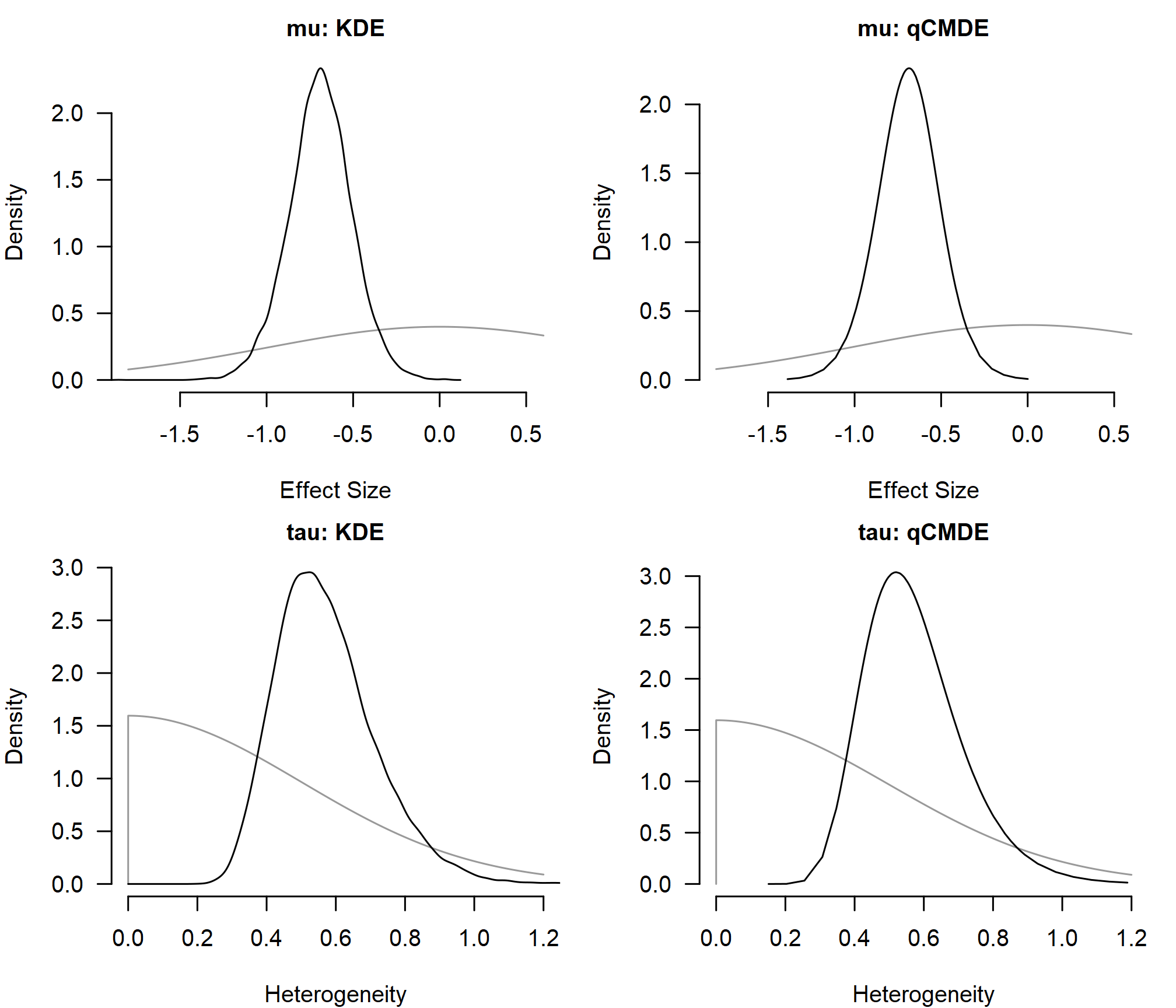

The qCMDE curves are smoother on both panels, but otherwise track the KDE summary in shape and location.

Testing the Mean Effect

Bayes factors compare two models by their prior predictive performance, usually through the ratio of marginal likelihoods (Kass & Raftery, 1995). For point-null hypotheses on a single parameter, the same Bayes factor can be obtained from the Savage–Dickey density ratio (Dickey, 1971; Wagenmakers et al., 2010), which needs only the prior and posterior density ordinate at the tested value. For inequality and region hypotheses, the encompassing-prior approach computes the Bayes factor as the change from prior odds to posterior odds for the restricted region (Klugkist et al., 2005). The Savage–Dickey and encompassing-prior routes are both available from a single fit through hypothesis(); the rest of this section walks through three example hypotheses on the average effect and contrasts both routes:

$\text{BF}_{10}$ : an unrestricted average effect against a point null at 0;
$\text{BF}_{-0}$ : a negative average effect against a point null at 0;
$\text{BF}_{-+}$ : a negative average effect against a positive average effect.

The posterior-based route uses hypothesis(). With density_method = "qCMDE", the point-null hypotheses use the qCMDE ordinate at 0 which improves stability of the estimate. The region test $\text{BF}_{-+}$ uses prior-posterior odds and does not need a density ordinate.

mu_posterior_bf <- hypothesis(
  fit_simple, density_method = "qCMDE",
  hypothesis     = c(
    "mu != 0",
    "mu < 0 vs mu = 0",
    "mu < 0 vs mu > 0"
  ),
)
mu_posterior_bf
#>  Alternative:  Null:       BF error%(BF)
#>       mu != 0 mu = 0   58.328     10.580
#>        mu < 0 mu = 0  116.610     10.580
#>        mu < 0 mu > 0 2499.000     40.834
#> qCMDE relative MCSE is 10.6% (requested precision target 5%). Higher precision can be obtained by increasing 'samples' in the 'density_control' argument.
#> qCMDE relative MCSE is 10.6% (requested precision target 5%). Higher precision can be obtained by increasing 'samples' in the 'density_control' argument.
#> qCMDE finite-population row-sampling relative error is 10.8% (requested precision target 5%). Higher precision can be obtained by increasing 'samples' in the 'density_control' argument.
#> qCMDE finite-population row-sampling relative error is 10.8% (requested precision target 5%). Higher precision can be obtained by increasing 'samples' in the 'density_control' argument.
#> qCMDE effective sample size is 70.7 (warning threshold 100).
#> qCMDE effective sample size is 70.7 (warning threshold 100).

The bridge sampling route fits one constrained model per hypothesis side, attaches marginal likelihoods with add_marglik(), and compares them with bf().

prior_effect_null     <- prior(distribution = "spike",  parameters = list(location = 0))
prior_effect_negative <- prior(distribution = "normal", parameters = list(mean = 0, sd = 1), truncation = list(lower = -Inf, upper = 0))
prior_effect_positive <- prior(distribution = "normal", parameters = list(mean = 0, sd = 1), truncation = list(lower = 0, upper = Inf))

fit_simple <- add_marglik(fit_simple)

fit_simple_mu_null <- brma(
  yi = yi, vi = vi, measure = "RR",
  prior_effect = prior_effect_null,
  data = dat, seed = 2
)
fit_simple_mu_null <- add_marglik(fit_simple_mu_null)

fit_simple_mu_negative <- brma(
  yi = yi, vi = vi, measure = "RR",
  prior_effect = prior_effect_negative,
  data = dat, seed = 3
)
fit_simple_mu_negative <- add_marglik(fit_simple_mu_negative)

fit_simple_mu_positive <- brma(
  yi = yi, vi = vi, measure = "RR",
  prior_effect = prior_effect_positive,
  data = dat, seed = 4
)
fit_simple_mu_positive <- add_marglik(fit_simple_mu_positive)

bf_10         <- bf(fit_simple, fit_simple_mu_null)
bf_minus_0    <- bf(fit_simple_mu_negative, fit_simple_mu_null)
bf_minus_plus <- bf(fit_simple_mu_negative, fit_simple_mu_positive)

The two routes answer the same questions through different computations. Bridge sampling compares separately fitted constrained models, while the posterior-based route reuses one fitted model and only needs the qCMDE ordinate at the tested value. The table reports the resulting Bayes factors and the corresponding error estimates in percentages.

Bayes factor estimates for the mean-effect hypotheses.
Test	Posterior BF	Bridge BF
$\text{BF}_{10}$	58.3	65.6
$\text{BF}_{-0}$	116.6	130.9
$\text{BF}_{-+}$	2499.0	2027.8

The point-null Bayes factors agree closely across the two routes. The posterior-based value for $\text{BF}_{-+}$ is limited by the number of posterior draws as only a very small proportion of samples is at the positive side. Consequently, the encompassing prior estimate is much more variable than the corresponding bridge sampling approach (see the the large error%(BF) reported earlier). In general, Bayes factors larger than 100 (lower than 1/100) are likely to have limited precision when using the posterior based or product-space approaches. (This usually does not matter for the interpretation, i.e., the data provide overwhelming evidence for one of the hypotheses.)

Meta-Regression

We next add absolute latitude (ablat) and allocation method (alloc) as moderators. For the categorical moderator we use mean-difference contrasts via set_contrast_factor_predictors = "meandif". It specifies the prior distribution such that the allocation levels are treated as exchangeable; the prior distribution does not depend on an arbitrary reference level and is better suited to hypothesis tests comparing allocation methods among each other.

fit_meta_reg <- brma(
  yi = yi, vi = vi, measure = "RR",
  mods = ~ ablat + alloc,
  set_contrast_factor_predictors = "meandif",
  prior_effect = prior_effect_normal,
  data = dat, seed = 5
)

summary(fit_meta_reg)
#> 
#> Bayesian Mixed-Effect Model (k = 13)
#> 
#> Common Estimates
#>      Mean    SD 0.025   0.5 0.975 error(MCMC) error(MCMC)/SD  ESS R-hat
#> tau 0.382 0.155 0.124 0.366 0.725     0.00249          0.016 3889 1.000
#> 
#> Meta-Regression
#>                          Mean    SD  0.025    0.5  0.975 error(MCMC) error(MCMC)/SD   ESS R-hat
#> intercept               0.188 0.333 -0.523  0.206  0.811     0.00296          0.009 12876 1.000
#> ablat                  -0.026 0.009 -0.043 -0.026 -0.005     0.00009          0.010 11011 1.000
#> alloc[dif: alternate]   0.073 0.205 -0.346  0.075  0.490     0.00186          0.009 12313 1.000
#> alloc[dif: random]     -0.174 0.174 -0.538 -0.166  0.152     0.00165          0.009 11253 1.000
#> alloc[dif: systematic]  0.101 0.192 -0.258  0.092  0.505     0.00166          0.009 13319 1.000

qCMDE is again available directly through plot.brma(). When interpreting categorical moderators, estimated marginal means (EMMs) are a clearer way to report the results. The marginal_means() allows us to compute Bayes factors using bf = TRUE and use the qCMDE via density_method = "qCMDE" arguments. The density estimate is directly saved in the EMMs object, so the corresponding hypotheses can be tested later with hypothesis().

emm_meta_reg_default <- marginal_means(fit_meta_reg)
emm_meta_reg_qcmde   <- marginal_means(fit_meta_reg, bf = TRUE, density_method = "qCMDE")

The four panels below compare KDE and qCMDE for the ablat coefficient and for the per-level posterior of the three alloc marginal means.

par(mfrow = c(2, 2), mar = c(4, 4, 2, 1), cex.axis = 0.8, cex.lab = 0.8, cex.main = 0.75)

plot(fit_meta_reg, parameter = "ablat", prior = TRUE, density_method = "KDE",   main = "KDE",   xlim = c(-0.08, 0.03))
plot(fit_meta_reg, parameter = "ablat", prior = TRUE, density_method = "qCMDE", main = "qCMDE", xlim = c(-0.08, 0.03))
plot(emm_meta_reg_default, parameter = "alloc", prior = TRUE, main = "alloc means: KDE",   xlim = c(-1.6, 0.3))
plot(emm_meta_reg_qcmde,   parameter = "alloc", prior = TRUE, main = "alloc means: qCMDE", xlim = c(-1.6, 0.3))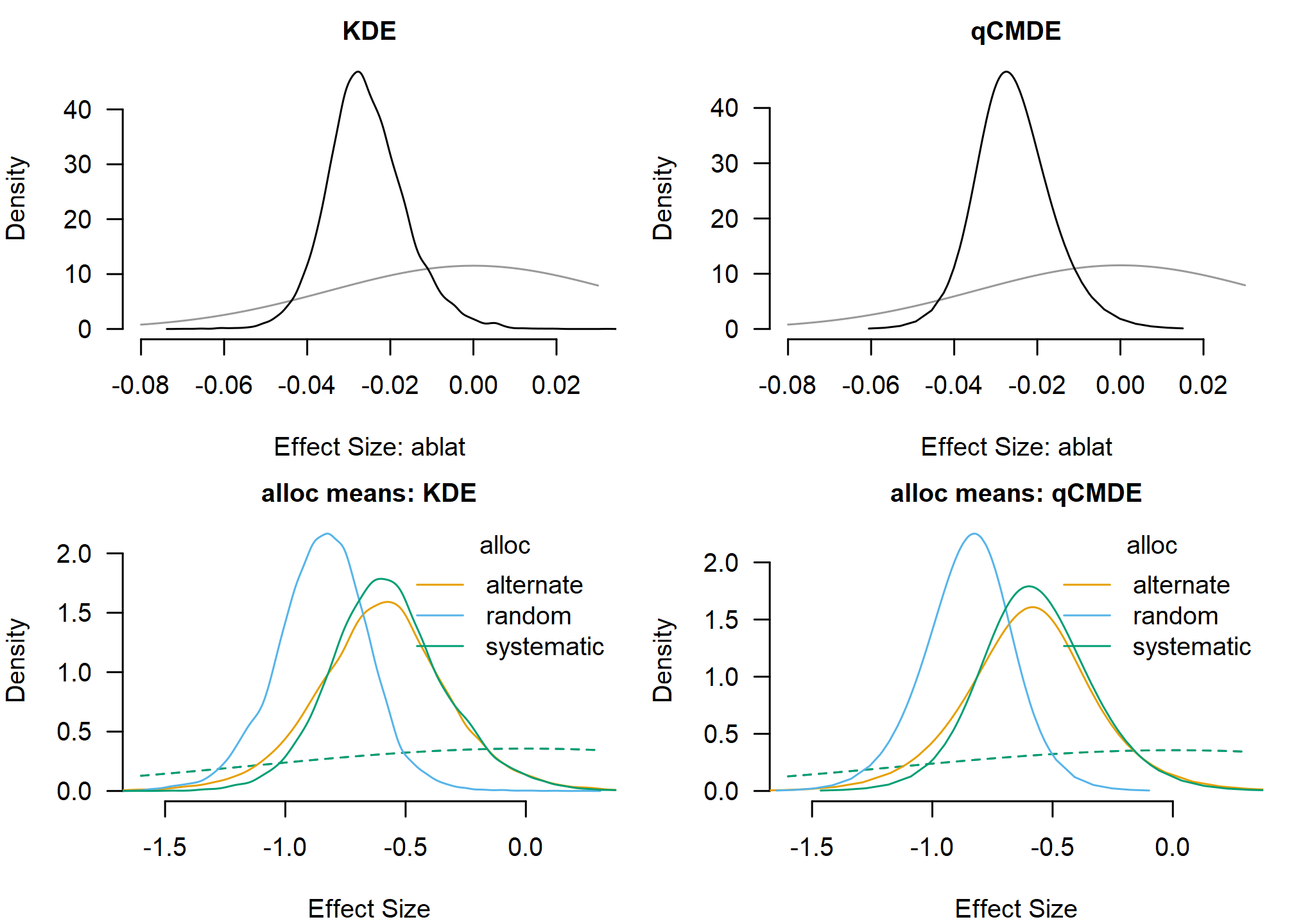

Hypotheses on the categorical moderator can then be stated directly in terms of named allocation-method marginal means. The bracket syntax (alloc[alternate]) selects a named level from the allocation marginal posterior.

hypothesis(
  emm_meta_reg_qcmde,
  hypothesis = c(
    "alloc[alternate] > alloc[random]",
    "alloc[alternate] > alloc[systematic]",
    "alloc[random] > alloc[systematic]"
  )
)
#>                                            Alternative:                                       Null:    BF error%(BF)
#> mu_alloc (1)     mu_alloc[alternate] > mu_alloc[random]     mu_alloc[alternate] <= mu_alloc[random] 3.808      2.012
#> mu_alloc (2) mu_alloc[alternate] > mu_alloc[systematic] mu_alloc[alternate] <= mu_alloc[systematic] 0.921      1.634
#> mu_alloc (3)    mu_alloc[random] > mu_alloc[systematic]    mu_alloc[random] <= mu_alloc[systematic] 0.212      2.148

References

Bartoš, F., & Maier, M. (2020). RoBMA: An R package for robust Bayesian meta-analyses. https://CRAN.R-project.org/package=RoBMA

Chen, M.-H. (1994). Importance-weighted marginal bayesian posterior density estimation. Journal of the American Statistical Association, 89(427), 818–824. https://doi.org/10.1080/01621459.1994.10476815

Dickey, J. M. (1971). The weighted likelihood ratio, linear hypotheses on normal location parameters. The Annals of Mathematical Statistics, 204–223. https://doi.org/10.1214/aoms/1177693507

Gelfand, A. E., Smith, A. F., & Lee, T.-M. (1992). Bayesian analysis of constrained parameter and truncated data problems using gibbs sampling. Journal of the American Statistical Association, 87(418), 523–532. https://doi.org/10.1080/01621459.1992.10475235

Gronau, Q. F., Sarafoglou, A., Matzke, D., Ly, A., Boehm, U., Marsman, M., Leslie, D. S., Forster, J. J., Wagenmakers, E.-J., & Steingroever, H. (2017). A tutorial on bridge sampling. Journal of Mathematical Psychology, 81, 80–97. https://doi.org/10.1016/j.jmp.2017.09.005

Kass, R. E., & Raftery, A. E. (1995). Bayes factors. Journal of the American Statistical Association, 90(430), 773–795. https://doi.org/10.1080/01621459.1995.10476572

Klugkist, I., Kato, B., & Hoijtink, H. (2005). Bayesian model selection using encompassing priors. Statistica Neerlandica, 59(1), 57–69. https://doi.org/10.1111/j.1467-9574.2005.00279.x

Lodewyckx, T., Kim, W., Lee, M. D., Tuerlinckx, F., Kuppens, P., & Wagenmakers, E.-J. (2011). A tutorial on Bayes factor estimation with the product space method. Journal of Mathematical Psychology, 55(5), 331–347. https://doi.org/10.1016/j.jmp.2011.06.001

Viechtbauer, W. (2010). Conducting meta-analyses in R with the metafor package. Journal of Statistical Software, 36(3), 1–48. https://doi.org/10.18637/jss.v036.i03

Wagenmakers, E.-J., Lodewyckx, T., Kuriyal, H., & Grasman, R. (2010). Bayesian hypothesis testing for psychologists: A tutorial on the savage–dickey method. Cognitive Psychology, 60(3), 158–189. https://doi.org/10.1016/j.cogpsych.2009.12.001

František Bartoš

25th of October 2026

Simple Meta-Analysis

qCMDE Posterior Density Estimation

Testing the Mean Effect

Meta-Regression

References