Location-Scale Meta-Analysis

This vignette illustrates how to fit location-scale meta-analytic models with the RoBMA R package (Bartoš & Maier, 2020). We walk through the writing-to-learn dataset (dat.bangertdrowns2004 in the metadat package), showing the brma() call with the scale = ~ ... argument alongside its metafor::rma() counterpart (Viechtbauer, 2010), and build from a simple random-effects model up to a model with different predictors in the location and scale parts.

A location-scale model parameterizes the between-study heterogeneity $\tau$ as a regression on study-level covariates, allowing $\tau$ to vary across subgroups or as a function of continuous moderators. The location side is the usual meta-regression on the effect.

All brma() calls keep the default prior distributions; see the Prior Distributions vignette for the prior definitions and customization options. For the non-location-scale workflow showing more features (also applicable to location-scale models) see the Bayesian Meta-Analysis vignette.

Random-Effects Model

The writing-to-learn dataset contains 48 standardized mean differences from studies on the effectiveness of school-based writing interventions on academic achievement. Effect sizes yi and sampling variances vi are already provided.

data("dat.bangertdrowns2004", package = "metadat")
dat <- dat.bangertdrowns2004
dat$ni100 <- dat$ni / 100
dat$meta  <- as.factor(dat$meta)
dat$imag  <- as.factor(dat$imag)

We start from a standard random-effects model with no scale predictor.

fit1_metafor <- metafor::rma(yi, vi, data = dat)
fit1_metafor
#> 
#> Random-Effects Model (k = 48; tau^2 estimator: REML)
#> 
#> tau^2 (estimated amount of total heterogeneity): 0.0499 (SE = 0.0197)
#> tau (square root of estimated tau^2 value):      0.2235
#> I^2 (total heterogeneity / total variability):   58.37%
#> H^2 (total variability / sampling variability):  2.40
#> 
#> Test for Heterogeneity:
#> Q(df = 47) = 107.1061, p-val < .0001
#> 
#> Model Results:
#> 
#> estimate      se    zval    pval   ci.lb   ci.ub      
#>   0.2219  0.0460  4.8209  <.0001  0.1317  0.3122  *** 
#> 
#> ---
#> Signif. codes:  0 '***' 0.001 '**' 0.01 '*' 0.05 '.' 0.1 ' ' 1

fit1_brma <- brma(
  yi = yi, vi = vi, measure = "SMD",
  data = dat, seed = 1
)

summary(fit1_brma, include_mcmc_diagnostics = FALSE)
#> 
#> Bayesian Random-Effects Model (k = 48)
#> 
#> Estimates
#>      Mean    SD 0.025   0.5 0.975
#> mu  0.220 0.048 0.130 0.220 0.317
#> tau 0.227 0.053 0.131 0.224 0.340

The pooled effect and the single heterogeneity parameter tau track the REML estimates from the metafor package.

Adding a Scale Predictor

Sample size is a natural candidate for explaining heterogeneity: smaller studies often produce more variable estimates than larger ones. We add the rescaled total sample size (ni100 = ni / 100) on both the location and the scale side.

fit2_metafor <- suppressWarnings(metafor::rma(
  yi, vi,
  mods  = ~ ni100,
  scale = ~ ni100,
  data = dat
))
fit2_metafor
#> 
#> Location-Scale Model (k = 48; tau^2 estimator: REML)
#> 
#> Test for Residual Heterogeneity:
#> QE(df = 46) = 95.1352, p-val < .0001
#> 
#> Test of Location Coefficients (coefficient 2):
#> QM(df = 1) = 7.8268, p-val = 0.0051
#> 
#> Model Results (Location):
#> 
#>          estimate      se     zval    pval    ci.lb    ci.ub      
#> intrcpt    0.3017  0.0661   4.5629  <.0001   0.1721   0.4313  *** 
#> ni100     -0.0553  0.0198  -2.7976  0.0051  -0.0940  -0.0165   ** 
#> 
#> Test of Scale Coefficients (coefficient 2):
#> QM(df = 1) = 3.1850, p-val = 0.0743
#> 
#> Model Results (Scale):
#> 
#>          estimate      se     zval    pval    ci.lb    ci.ub     
#> intrcpt   -1.9209  0.6690  -2.8713  0.0041  -3.2321  -0.6097  ** 
#> ni100     -0.9174  0.5141  -1.7847  0.0743  -1.9250   0.0901   . 
#> 
#> ---
#> Signif. codes:  0 '***' 0.001 '**' 0.01 '*' 0.05 '.' 0.1 ' ' 1

fit2_brma <- brma(
  yi = yi, vi = vi, measure = "SMD",
  mods  = ~ ni100,
  scale = ~ ni100,
  data = dat, seed = 1
)

summary(fit2_brma, include_mcmc_diagnostics = FALSE)
#> 
#> Bayesian Location-Scale Model (k = 48)
#> 
#> Location
#>             Mean    SD  0.025    0.5  0.975
#> intercept  0.303 0.068  0.171  0.302  0.437
#> ni100     -0.056 0.023 -0.103 -0.056 -0.013
#> 
#> Scale
#>                  Mean    SD  0.025    0.5 0.975
#> exp(intercept)  0.348 0.118  0.148  0.338 0.608
#> ni100          -0.375 0.225 -0.865 -0.366 0.042
#> exp(Intercept) corresponds to the between-study heterogeneity tau; the meta-regression coefficients correspond to the multiplicative effects on log-scale.

The location coefficient on ni100 matches the REML estimate from the metafor package. The scale block reports exp(intercept), which is the baseline between-study heterogeneity $\tau$ , and a multiplicative log-scale coefficient on ni100. Note that metafor::rma() regresses $\log(\tau^2)$ while brma() regresses $\log(\tau)$ , so each metafor package scale coefficient is exactly twice the matching brma() coefficient.

regplot() with pi = TRUE overlays the prediction interval on the bubble plot. Because $\tau$ varies with ni100, the brma() prediction band narrows toward larger sample sizes, where the model expects less between-study heterogeneity. metafor::regplot() does not currently draw a prediction interval for location-scale models, so only the regression line and confidence band appear in the left panel.

par(mfrow = c(1, 2), mar = c(4, 4, 2, 1), cex.axis = 0.8, cex.lab = 0.8, cex.main = 0.75)
metafor::regplot(fit2_metafor, mod = "ni100", pi = TRUE,
                 main = "metafor", xlim = c(0, 6), ylim = c(-1, 2))
regplot(fit2_brma, mod = "ni100", pi = TRUE,
        main = "RoBMA",   xlim = c(0, 6), ylim = c(-1, 2))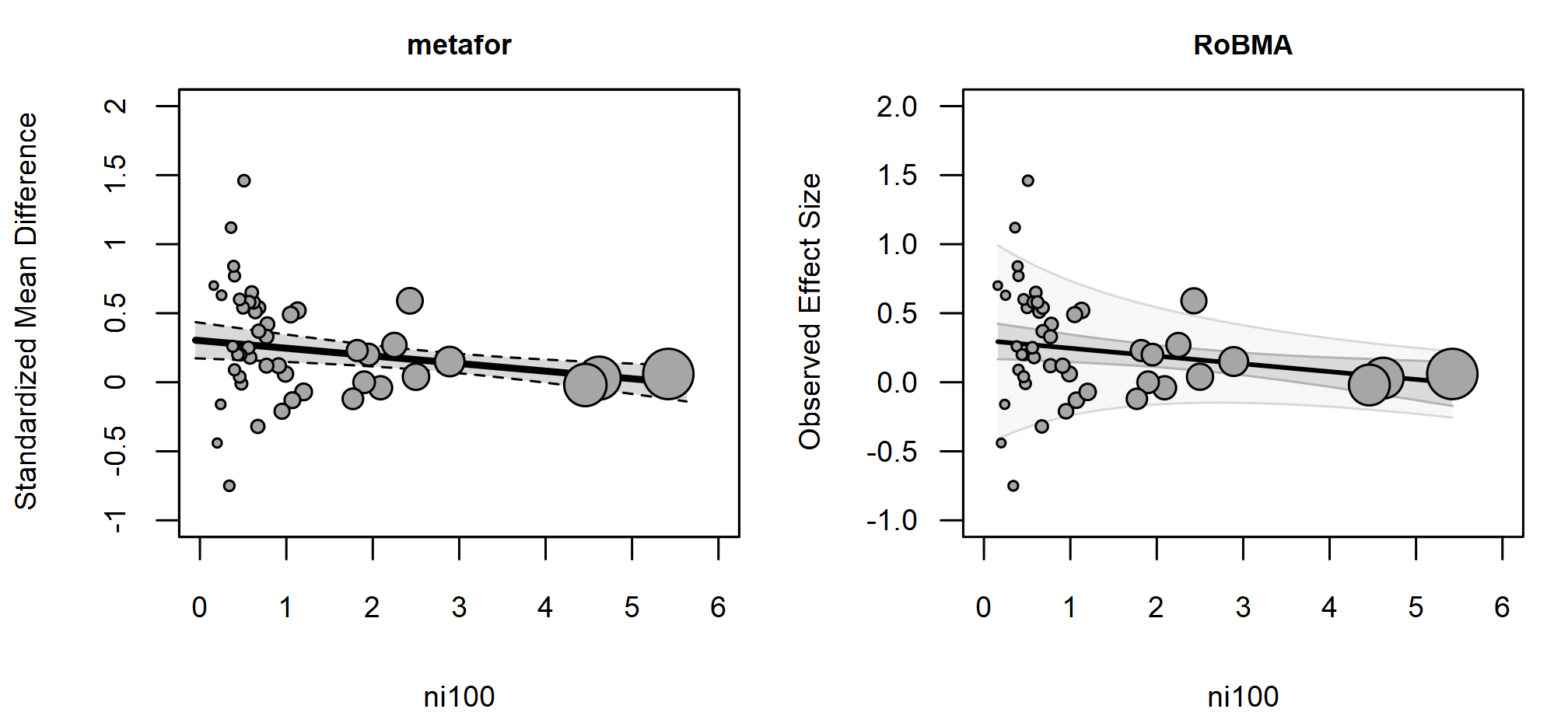

Different Variables in Location and Scale

Variables in the location and scale parts can differ. The next fit adds metacognitive reflection (meta) on the location side and imaginative-component coding (imag) on the scale side.

fit3_metafor <- suppressWarnings(metafor::rma(
  yi, vi,
  mods  = ~ ni100 + meta,
  scale = ~ ni100 + imag,
  data = dat
))
fit3_metafor
#> 
#> Location-Scale Model (k = 46; tau^2 estimator: REML)
#> 
#> Test for Residual Heterogeneity:
#> QE(df = 43) = 82.2711, p-val = 0.0003
#> 
#> Test of Location Coefficients (coefficients 2:3):
#> QM(df = 2) = 12.4826, p-val = 0.0019
#> 
#> Model Results (Location):
#> 
#>          estimate      se     zval    pval    ci.lb    ci.ub      
#> intrcpt    0.2303  0.0655   3.5166  0.0004   0.1019   0.3586  *** 
#> ni100     -0.0565  0.0188  -3.0113  0.0026  -0.0933  -0.0197   ** 
#> meta1      0.1469  0.0690   2.1305  0.0331   0.0118   0.2820    * 
#> 
#> Test of Scale Coefficients (coefficients 2:3):
#> QM(df = 2) = 5.0289, p-val = 0.0809
#> 
#> Model Results (Scale):
#> 
#>          estimate      se     zval    pval    ci.lb    ci.ub     
#> intrcpt   -2.3456  0.8354  -2.8079  0.0050  -3.9829  -0.7084  ** 
#> ni100     -0.9995  0.6087  -1.6421  0.1006  -2.1925   0.1935     
#> imag1      2.1258  1.1857   1.7929  0.0730  -0.1981   4.4497   . 
#> 
#> ---
#> Signif. codes:  0 '***' 0.001 '**' 0.01 '*' 0.05 '.' 0.1 ' ' 1

fit3_brma <- brma(
  yi = yi, vi = vi, measure = "SMD",
  mods  = ~ ni100 + meta,
  scale = ~ ni100 + imag,
  data = dat, seed = 1
)

summary(fit3_brma, include_mcmc_diagnostics = FALSE)
#> 
#> Bayesian Location-Scale Model (k = 46)
#> 
#> Location
#>             Mean    SD  0.025    0.5  0.975
#> intercept  0.229 0.069  0.095  0.228  0.369
#> ni100     -0.058 0.023 -0.106 -0.058 -0.016
#> meta[1]    0.173 0.078  0.026  0.171  0.336
#> 
#> Scale
#>                  Mean    SD  0.025    0.5 0.975
#> exp(intercept)  0.291 0.113  0.100  0.281 0.542
#> ni100          -0.338 0.237 -0.826 -0.333 0.108
#> imag[1]         0.361 0.447 -0.600  0.383 1.180
#> exp(Intercept) corresponds to the between-study heterogeneity tau; the meta-regression coefficients correspond to the multiplicative effects on log-scale.

Each scale coefficient is again roughly half of its metafor package counterpart, with brma() shrinking the larger metafor package estimates more strongly because of the weakly informative default prior distribution.

Scale Predictor Prior Distributions

Scale regression coefficients are not on the effect-size scale: they describe multiplicative changes in $\tau$ on the log scale and are therefore scale-free. The default prior distribution is Normal(0, 0.5), which corresponds to a weakly informative prior distribution on the multiplicative effect. A coefficient of $\pm 0.5$ corresponds to roughly $\exp(\pm 0.5) \approx 0.6$ or $1.65$ , i.e., a $40\%$ decrease or $65\%$ increase in $\tau$ per unit change in the predictor; values past $\pm 1$ correspond to a halving or doubling, which the prior distribution treats as extreme.

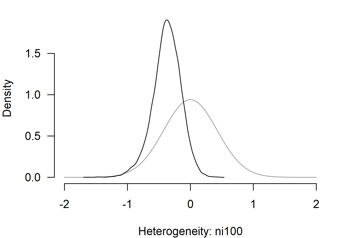
plot() with prior = TRUE overlays the prior distribution on the posterior so the shift is visible. parameter_scale = "ni100" selects the scale-side coefficient (the analogous selector on the location side is parameter_mods = "ni100").

par(mar = c(4, 4, 1, 1))
plot(fit2_brma, parameter_scale = "ni100", prior = TRUE, xlim = c(-2, 2))

Other Inference Helpers

All inference helpers available for any other brma() fit work the same way for the location-scale fit specified via scale = ~ .... This includes meta-regression bubble plots, marginal means, model comparison via Bayes factors, multilevel structures via cluster, and the full set of model-fit diagnostics. See the Bayesian Meta-Analysis vignette for more details.

References

Bartoš, F., & Maier, M. (2020). RoBMA: An R package for robust Bayesian meta-analyses. https://CRAN.R-project.org/package=RoBMA

Viechtbauer, W. (2010). Conducting meta-analyses in R with the metafor package. Journal of Statistical Software, 36(3), 1–48. https://doi.org/10.18637/jss.v036.i03