Creates a prior distribution for PET or PEESE models

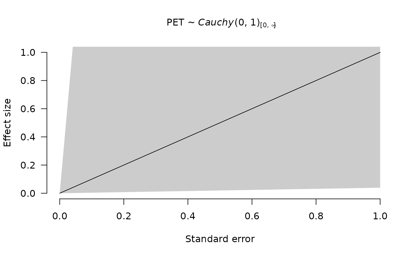
prior creates a prior distribution for fitting a PET or PEESE style models in RoBMA. The prior distribution can be visualized by the plot function.

prior_PET(
  distribution,
  parameters,
  truncation = list(lower = 0, upper = Inf),
  prior_weights = 1
)

prior_PEESE(
  distribution,
  parameters,
  truncation = list(lower = 0, upper = Inf),
  prior_weights = 1
)

Arguments

distribution

name of the prior distribution. The possible options are

"point"

for a point density characterized by a location parameter.

"normal"

for a normal distribution characterized by a mean and sd parameters.

"lognormal"

for a lognormal distribution characterized by a meanlog and sdlog parameters.

"cauchy"

for a Cauchy distribution characterized by a location and scale parameters. Internally converted into a generalized t-distribution with df = 1.

"t"

for a generalized t-distribution characterized by a location, scale, and df parameters.

"gamma"

for a gamma distribution characterized by either shape and rate, or shape and scale parameters. The latter is internally converted to the shape and rate parametrization

"invgamma"

for an inverse-gamma distribution characterized by a shape and scale parameters. The JAGS part uses the BayesTools module distribution dbt_invgamma(shape, scale) on the natural parameter.

"beta"

for a beta distribution characterized by an alpha and beta parameters.

"exp"

for an exponential distribution characterized by either rate or scale parameter. The later is internally converted to rate.

"uniform"

for a uniform distribution defined on a range from a to b

"moment"

for a Johnson-Rossell moment prior characterized by exactly one of mode or tau, an optional order that defaults to 1, and an optional location that defaults to 0.

"invmoment"

for a Johnson-Rossell inverse-moment prior characterized by exactly one of mode or tau, a df, an optional order that defaults to 1, and an optional location that defaults to 0.

"dirichlet"

for a Dirichlet distribution over a simplex, whose finite nonnegative coordinates must have a finite total and roundoff bound and sum to one within that bound, characterized by a concentration vector alpha. Numeric entries must be finite and at least 0.01; this is a supported-input minimum, not a numerical guarantee. Positive expression-valued concentrations retain their existing JAGS-only support: expression containers, including literal elements, are not statically evaluated or validated, and R random generation refuses them. Cumulative weight functions and ordered allocations require numeric concentrations. Accepted sampling can still be unavailable; see prior_functions. Two-bin cumulative JAGS initialization near the minimum can repeatedly refuse unrepresentable interior ratios. Density and plot methods show one beta marginal per simplex coordinate.

parameters

list of appropriate parameters for a given distribution.

truncation

list with two elements, lower and upper, that define the lower and upper truncation of the distribution. Defaults to list(lower = -Inf, upper = Inf). The truncation is automatically set to the bounds of the support.

prior_weights

prior odds associated with a given distribution. The value is passed into the model fitting function, which creates models corresponding to all combinations of prior distributions for each of the model parameters and sets the model priors odds to the product of its prior distributions.

Value

prior_PET and prior_PEESE return an object of class 'prior'.

See also

plot.prior(), prior()

Examples

# create a half-Cauchy prior distribution
# (PET and PEESE specific functions automatically set lower truncation at 0)
p1 <- prior_PET(distribution = "Cauchy", parameters = list(location = 0, scale = 1))

plot(p1)