Plots a prior object

# S3 method for class 'prior'
plot(
  x,
  plot_type = "base",
  x_seq = NULL,
  xlim = NULL,
  x_range_quant = NULL,
  n_points = 1000,
  n_samples = 10000,
  force_samples = FALSE,
  transformation = NULL,
  transformation_arguments = NULL,
  transformation_settings = FALSE,
  show_figures = if (individual) -1 else NULL,
  individual = FALSE,
  rescale_x = FALSE,
  par_name = NULL,
  ...
)

Arguments

x

a prior

plot_type

whether to use a base plot "base" or ggplot2 "ggplot" for plotting.

x_seq

sequence of x coordinates

xlim

x plotting range

x_range_quant

quantile used for automatically obtaining x_range if both x_range and x_seq are unspecified. A number in the open interval (0, 0.5); other values are refused. Defaults to 0.005 for all but Cauchy, Student-t, Gamma, inverse-gamma, moment, and inverse-moment distributions that use 0.010.

n_points

number of equally spaced points in the x_range if x_seq is unspecified

n_samples

number of samples from the prior distribution if the density cannot be obtained analytically (or if samples are forced with force_samples = TRUE)

force_samples

should prior be sampled instead of obtaining analytic solution whenever possible. For supported ordered mixed measures, exact analytic curves and atoms are retained and the requested samples are attached to each component. Supported scalar ordered literal point totals and mixtures whose total components are all literal points do not sample, store draws, or advance the RNG when force_samples = FALSE. With force_samples = TRUE, their original seeded draws are attached without replacing the analytic measure. Other ordered families retain their existing sampling fallback.

transformation

transformation to be applied to the prior distribution. Either a character specifying one of the prepared transformations:

lin: linear transformation in form of a + b*x
tanh: hyperbolic tangent transformation
exp: exponential transformation

, or a list containing the transformation function fun, inverse transformation function inv, and derivative of the transformation jac, evaluated on the original support. A custom transformation can also declare output_support = c(lower, upper). Display grids on the transformed scale are evaluated only within these bounds; a wider plotting range is retained without extending the density. Infinite inverse values at support boundaries are omitted from continuous density grids. Point masses retain their transformed locations.

transformation_arguments

a list with named arguments for the transformation

transformation_settings

boolean indicating whether the explicitly supplied x_seq or x_range is on the transformed scale. Automatically selected prior-coordinate ranges are always obtained on the source scale before the density family's existing transformation handling.

show_figures

which figures should be returned in case of multiple plots are generated. Useful when priors for the omega parameter are plotted and individual = TRUE. For weight functions plotted individually by plot.prior() and plot_posterior(), figure k shows the publication weight omega of the k-th p-value interval in ascending order, the order in which summary tables (including RoBMA's) print the omegas; figure 1 is the reference weight of the most significant interval. In plot.prior(), a negative k omits figure -k (the default -1 omits the reference weight fixed at 1). For a two-sided weight function prior, the intervals are its two-sided p-value bins; tables on the one-sided p-value scale print these weights first and then repeat them for the mirrored intervals.

individual

should individual densities be returned (e.g., in case of weightfunction)

rescale_x

allows to rescale x-axis in case a weightfunction is plotted.

par_name

a type of parameter for which the prior is specified. Only relevant if the prior corresponds to a mu parameter that needs to be transformed.

...

additional graphical arguments. For mixed continuous and point distributions, ylim controls the density axis, ylim2 controls the probability-mass axis, and ylab2 controls its label.

Value

plot.prior returns either NULL or an object of class 'ggplot' if plot_type is plot_type = "ggplot". Dirichlet simplex priors are plotted as one beta marginal per coordinate; the ggplot method returns a list unless a single figure is selected. Ordered ggplot results use the original figure indices: a multiple-figure selection returns a list through the largest selected index, with NULL entries for unselected figures, including the default reference level. A bare ggplot is returned only when exactly one figure is selected; a selection of several figures always returns a positional list, even if one figure is visible. For an ordered level with mixed probability measure, the continuous density and exact probability-mass arrows are drawn together without rescaling either component. For ordered and Dirichlet simplex priors, show_figures holds non-zero integers within the number of figures that are all positive (select) or all negative (omit); other values stop with an error before any figure is drawn. Individual weight functions take a single figure.

Details

Declared point locations whose transformation images are not representable stop with BayesTools_transformation_image_unavailable, parent BayesTools_transformation. Its call is NULL and its transformation, source_values and images fields identify the matched failing finite entries; see posterior_transform(). Automatic prior-coordinate limits are selected on the source scale before transformation, regardless of transformation_settings. An endpoint with an infinite image uses the existing marginal tail convention described in density.prior(). Explicit xlim and x_seq retain their supplied source or transformed interpretation.

Ordered prior plots retain the continuous density of every non-reference level, including priors with an infinite density at an exact point. Only nonfinite plotting ordinates are omitted; finite ordinates and declared point masses are unchanged. An infinite density point is not a probability mass. This display rule also applies to lines.prior() and geom_prior() and leaves density.prior() and prior_density_ordinate() unchanged. Unknown or unsupported density routes keep their existing limitations. Simple priors, the marginals of simplex priors and individual omegas follow the same rule: nonfinite ordinates (such as the infinite density of a Gamma(0.5, 1) prior at zero) are not drawn, and the density axis ends at the largest finite ordinate. A curve without any finite ordinate stops with class BayesTools_prior_curve_unavailable; choose another xlim. Direct ordered plots and layers omit persisted zero-design reference levels from the default selection. Explicit selectors retain the original level numbering and can select a reference level. Genuine non-reference zero and point levels remain visible. Finite displayed peak heights depend on the evaluation grid and do not represent an infinite mathematical peak. A direct ordered curve with no finite plotting ordinate stops with class BayesTools_prior_curve_unavailable (also BayesTools_plot_condition); supply x_seq containing finite density ordinates. Probability-axis mapping and clipping checks use selected components only, including an explicitly selected reference.

Examples

# create some prior distributions
p0 <- prior(distribution = "point",  parameters = list(location = 0))
p1 <- prior(distribution = "normal", parameters = list(mean = 0, sd = 1))
p2 <- prior(distribution = "normal", parameters = list(mean = 0, sd = 1), truncation = list(0, Inf))

# a default plot
plot(p0)


# manipulate line thickness and color, change the parameter name
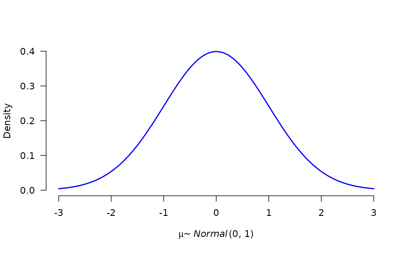
plot(p1, lwd = 2, col = "blue", par_name = bquote(mu))


# use ggplot
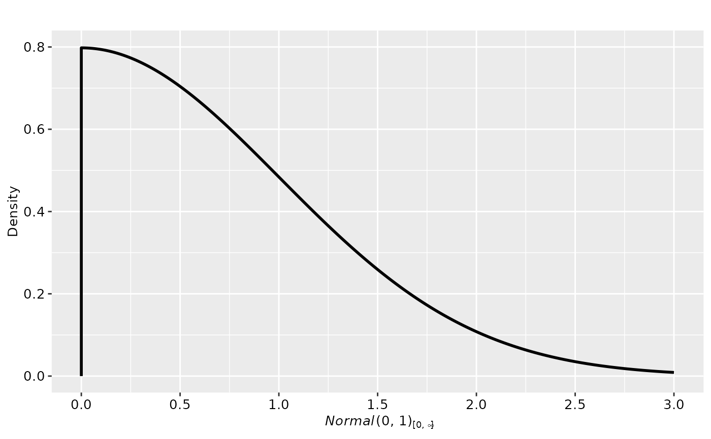
plot(p2, plot_type = "ggplot")


# utilize the ggplot prior geom
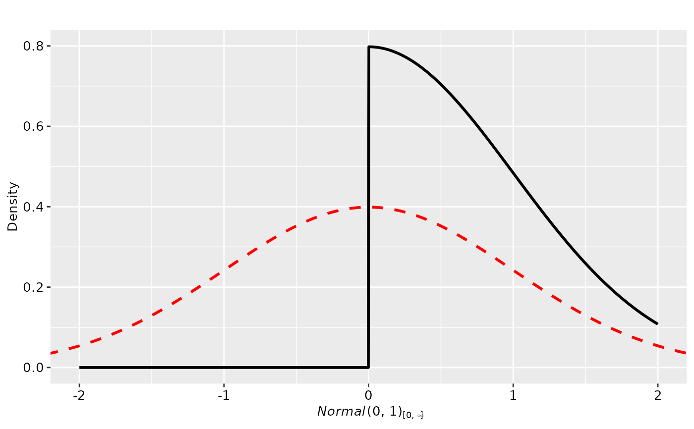
plot(p2, plot_type = "ggplot", xlim = c(-2, 2)) + geom_prior(p1, col = "red", lty = 2)


# apply transformation
plot(p1, transformation = "exp")

Plots a prior object

Arguments

Value

Details

See also

Examples