Fit a z-curve

zcurve is used to fit z-curve models. The function takes input of z-statistics or two-sided p-values and returns object of class "zcurve" that can be further interrogated by summary and plot function. It default to EM model, but different version of z-curves can be specified using the method and control arguments. See 'Examples' and 'Details' for more information.

zcurve(
  z,
  z.lb,
  z.ub,
  p,
  p.lb,
  p.ub,
  data,
  method = "EM",
  bootstrap = 1000,
  parallel = FALSE,
  control = NULL
)

Arguments

z

a vector of z-scores.

z.lb

a vector with start of censoring intervals of censored z-scores.

z.ub

a vector with end of censoring intervals of censored z-scores.

p

a vector of two-sided p-values, internally transformed to z-scores.

p.lb

a vector with start of censoring intervals of censored two-sided p-values.

p.ub

a vector with end of censoring intervals of censored two-sided p-values.

data

an object created with zcurve_data() function.

method

the method to be used for fitting. Possible options are Expectation Maximization "EM" and density "density", defaults to "EM".

bootstrap

the number of bootstraps for estimating CI. To skip bootstrap specify FALSE.

parallel

whether the bootstrap should be performed in parallel. Defaults to FALSE. The implementation is not completely stable and might cause a connection error.

control

additional options for the fitting algorithm more details in control EM or control density.

Value

The fitted z-curve object

Details

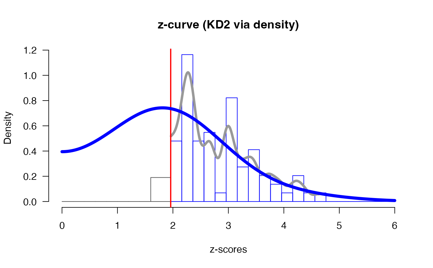
The function returns the EM method by default and changing method = "density" gives the KD2 version of z-curve as outlined in Bartoš and Schimmack (2020) . For the original z-curve (Brunner and Schimmack 2020) , referred to as KD1, specify 'control = "density", control = list(model = "KD1")'.

References

Bartoš F, Schimmack U (2020). “Z-curve. 2.0: Estimating Replication Rates and Discovery Rates.” doi:10.31219/osf.io/wr93f , submitted for publication.

Brunner J, Schimmack U (2020). “Estimating population mean power under conditions of heterogeneity and selection for significance.” Meta-Psychology, 4. doi:10.15626/MP.2018.874 .

See also

summary.zcurve(), plot.zcurve(), control_EM, control_density

Examples

# load data from OSC 2015 reproducibility project
OSC.z
#>  [1]  2.409175  3.245251  2.164192  3.191229  2.702059  3.137051  8.402858
#>  [8]  3.718460  4.293275  3.512496  1.973777  7.066053  4.383039  3.536266
#> [15]  3.392537  2.194877  3.059374  4.637228  3.982280  2.169338  1.946709
#> [22]  2.268213  4.180570  3.459550  3.731395  1.836848  3.100000 10.000000
#> [29]  2.967738  2.183487  2.408916  2.365618  2.257129  1.968592  3.909901
#> [36]  2.273435 10.000000  2.307984  2.290368  2.967738  2.014091 10.000000
#> [43] 10.000000  3.290527  2.432379  2.014091  2.575829 10.000000  2.307984
#> [50]  2.967738  2.967738  1.792831  3.290527  1.959964  2.297408  2.053749
#> [57] 10.000000  2.542699  2.403655 10.000000  3.410733  2.975294  3.849639
#> [64] 10.000000  2.273435  2.106589  3.694892  2.195944  2.307984  4.178900
#> [71]  1.951480  2.967738  2.226212  2.290368  2.967738  2.780638  2.612054
#> [78] 10.000000  2.652070 10.000000  2.725494  2.652070  3.042724  2.652070
#> [85]  2.970656  2.257129  2.386708  3.403461  2.120072  2.688852

# fit an EM z-curve (with disabled bootstrap due to examples times limits)
m.EM <- zcurve(OSC.z, method = "EM", bootstrap = FALSE)
# a version with 1000 boostraped samples would looked like:
m.EM <- zcurve(OSC.z, method = "EM", bootstrap = 1000)

# or KD2 z-curve (use larger bootstrap for real inference)
m.D <- zcurve(OSC.z, method = "density", bootstrap = FALSE)

# inspect the results
summary(m.EM)
#> Call:
#> zcurve(z = OSC.z, method = "EM", bootstrap = 1000)
#> 
#> model: EM via EM
#> 
#>     Estimate  l.CI  u.CI
#> ERR    0.615 0.455 0.748
#> EDR    0.383 0.075 0.698
#> 
#> Model converged in 28 + 195 iterations
#> Fitted using 73 z-values. 90 supplied, 85 significant (ODR = 0.94, 95% CI [0.87, 0.98]).
#> Q = -60.61, 95% CI[-72.01, -47.30]
summary(m.D)
#> Call:
#> zcurve(z = OSC.z, method = "density", bootstrap = FALSE)
#> 
#> model: KD2 via density
#> 
#>     Estimate
#> ERR    0.613
#> EDR    0.506
#> 
#> Model converged in 47 iterations
#> Fitted using 73 z-values. 90 supplied, 85 significant (ODR = 0.94, 95% CI [0.87, 0.98]).
#> RMSE = 0.11
# see '?summary.zcurve' for more output options

# plot the results
plot(m.EM)

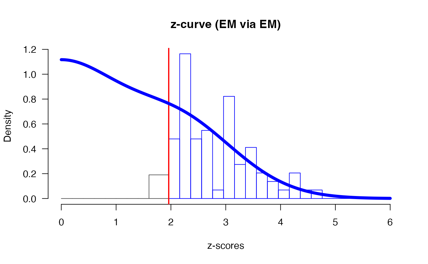plot(m.D)

# see '?plot.zcurve' for more plotting options

# to specify more options, set the control arguments
# ei. increase the maximum number of iterations and change alpha level
ctr1 <- list(
  "max_iter" = 9999,
  "alpha"    = .10
  )
if (FALSE) m1.EM <- zcurve(OSC.z, method = "EM", bootstrap = FALSE, control = ctr1)
# see '?control_EM' and '?control_density' for more information about different
# z-curves specifications